LSTM은 RNN의 단점이었던 장기의존성(time이 지날수록 gradient가 vanishing 하는 문제)을 해결함. 하지만 RNN에 비해서 모델 구조가 지나치게 복잡하다는 단점이 존재. GRU는 모델의 형태도 간단하지만 동시에 장기의존성 문제 또한 해결함.
이전은 전부 동일, torch의 GRU는 (input_size, hidden_size, num_layers)를 input으로 받음
1. 모델 구조
class GRU(nn.Module):

    def __init__(self, input_size, hidden_size, sequence_length, num_layers, device):
        super(GRU, self).__init__()
        self.device = device
        self.hidden_size = hidden_size
        self.num_layers = num_layers
        self.gru = nn.GRU(input_size, hidden_size, num_layers, batch_first=True)
        self.fc = nn.Linear(hidden_size*sequence_length, 1)

    def forward(self, x): # LSTM과는 달리 cell state가 다시 사라짐
        h0 = torch.zeros(self.num_layers, x.size()[0], self.hidden_size).to(self.device)
        out, _ = self.gru(x, h0) # cell state가 없음
        out = out.reshape(out.shape[0], -1) # <- state 추가
        out = self.fc(out)
        return out

# model
model = GRU(input_size=input_size,
                   hidden_size=hidden_size,
                   sequence_length=sequence_length,
                   num_layers=num_layers, device=device)

model = model.to(device)

# criterion, learning rate, epochs, optimizer 생성
criterion = nn.MSELoss()
lr = 1e-3
num_epochs = 201
optimizer = optim.Adam(model.parameters(), lr=lr)
2. Train 및 시각화
loss_graph = []
n = len(train_loader)
for epoch in range(num_epochs):
    running_loss = 0.0

    for i, data in enumerate(train_loader, 0):

        seq, target = data # 배치 데이터
        out = model(seq)
        loss = criterion(out, target)

        optimizer.zero_grad()
        loss.backward()
        optimizer.step()
        running_loss += loss.item()

    loss_graph.append(running_loss/n)
    if epoch % 100 == 0:
        print('[epoch: %d] loss: %.4f' %(epoch, running_loss/n))

# 시각화
plt.figure(figsize=(20,10))
plt.plot(loss_graph)
plt.show() 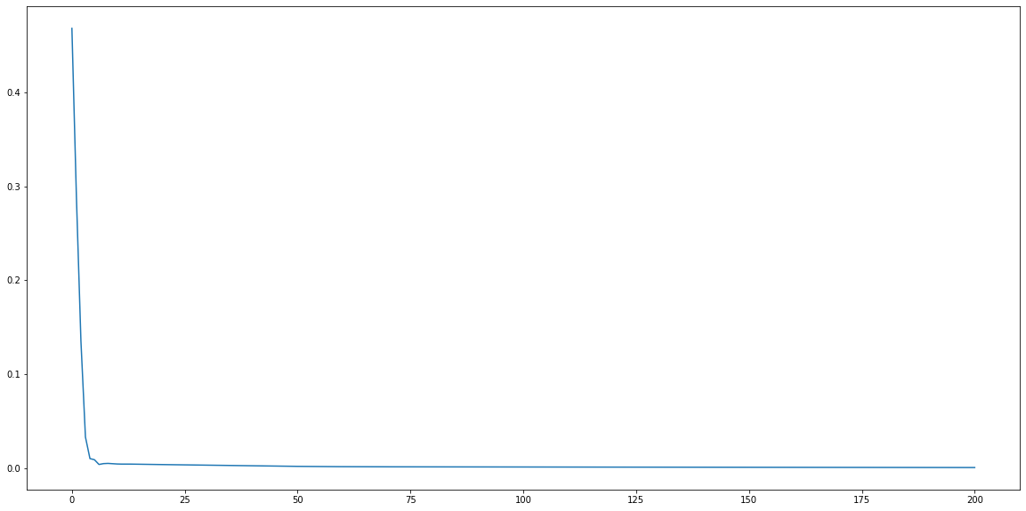
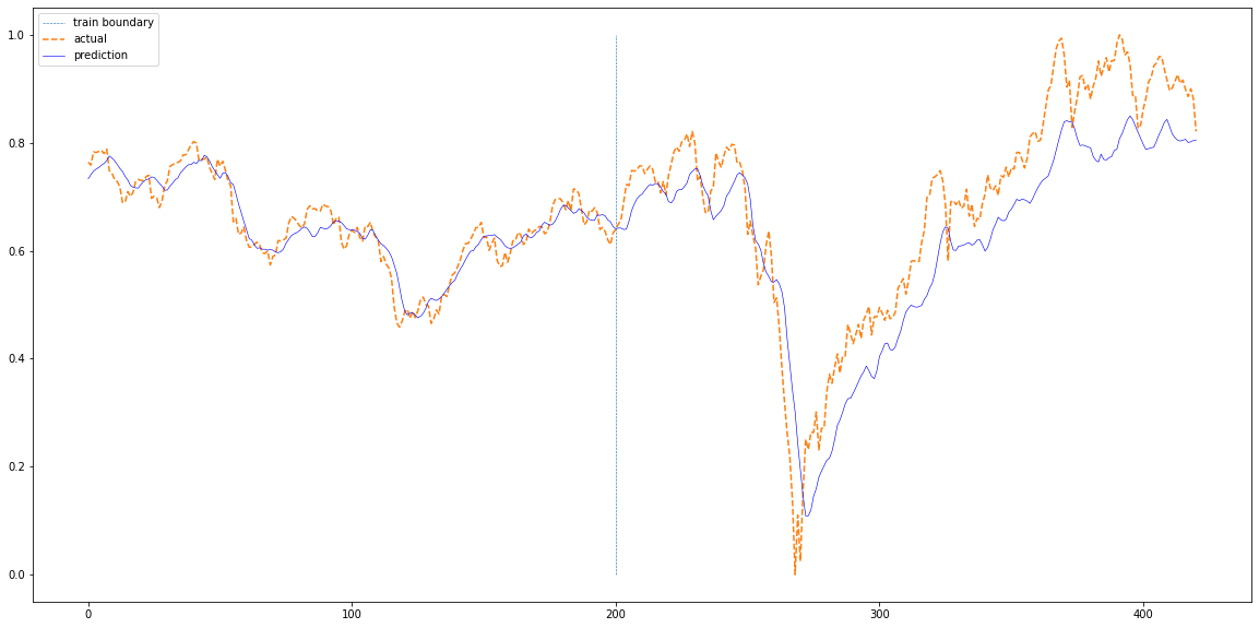
3. 실제 데이터와 비교
def plotting(train_loader, test_loader, actual):
    with torch.no_grad():
        train_pred = []
        test_pred = []

        for data in train_loader:
            seq, target = data # 배치 데이터
            #print(seq.size())
            out = model(seq)
            train_pred += out.cpu().numpy().tolist()

        for data in test_loader:
            seq, target = data # 배치 데이터
            #print(seq.size())
            out = model(seq)
            test_pred += out.cpu().numpy().tolist()
    total = train_pred+test_pred
    plt.figure(figsize=(20,10))
    plt.plot(np.ones(100)*len(train_pred),np.linspace(0,1,100),'--', linewidth=0.6)
    plt.plot(actual,'--')
    plt.plot(total,'b', linewidth=0.6)


    plt.legend(['train boundary','actual','prediction'])
    plt.show()

plotting(train_loader, test_loader, df['Close'][sequence_length:].values)
결론: GRU는 LSTM보다 학습에 사용될 게이트와 파라미터가 적은 구조(==RNN과 유사)이기 때문에 빠른 학습 속도가 장점. 하지만 LSTM 과 유사한 성능을 보여줌
--> GRU는 RNN과 비슷한 구조이지만 (간단하지만) 성능은 LSTM 급
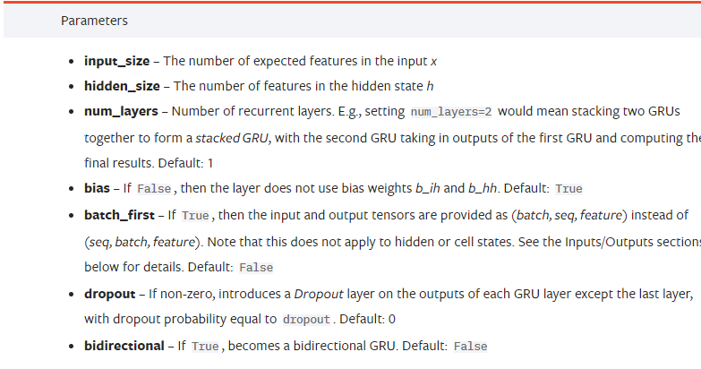
1. GRU의 parameter (input size = 변수 개수)
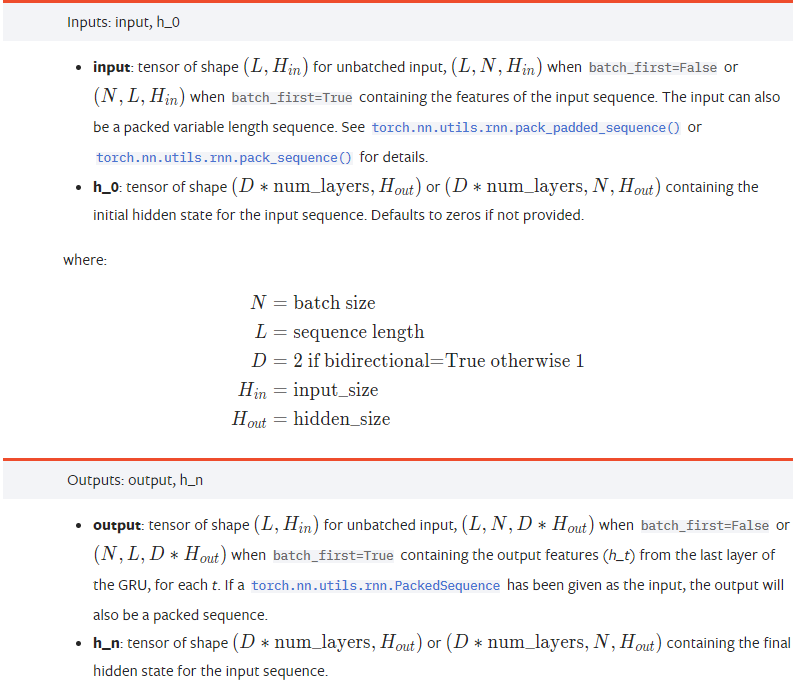
2. GRU의 input & output

pppanghyun