비즈니스 데이터 분석
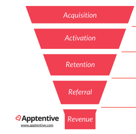
AARRR
AARRR은 시장 진입 단계에 맞는 특정 지표를 기준으로 우리 서비스의 상태를 가늠할 수 있는 효율적인 기준이다.
수 많은 데이터 중 현 시점에서 가장 핵심적인 지표에 집중할 수 있게 함으로써 분석할 리소스가 충분하지 않은 스타트업에게 매력적인 프레임워크
- Acquisition : 어떻게 우리 서비스를 접하였나
- Activation : 처음 서비스를 이용할 때 긍정적인 경험을 제공하는가
- Retention : 이후의 서비스 재사용률
- Referral : 사용자가 공유를 하고 있는가
- Revenue : 매출로 연결이 되고 있는가
Cohort analysis
- 코호트 분석은 분석 전에 데이터 세트의 데이터를 관련 그룹으로 나누는 일종의 행동 분석
- 이러한 그룹 또는 집단은 일반적으로 정의된 시간 범위 내에서 공통된 특성이나 경험을 공유
- 코호트 분석을 통해 회사는 고객이 겪는 자연적 주기를 고려하지 않고 맹목적으로 모든 고객을 분할하는 대신 고객의 수명 주기 전반에 걸쳐 패턴을 명확하게 볼 수 있음
- 이러한 시간 패턴을 보고 회사는 특정 집단에 맞게 서비스를 조정 가능
코호트 분석의 유형
- 📍 시간 집단
: 특정 기간 동안 제품이나 서비스에 가입한 고객
✅ 이러한 집단을 분석하면 고객이 회사의 제품이나 서비스를 사용하기 시작한 시점을 기준으로 고객의 행동이 나타난다.
시간은 월별 또는 분기별 또는 매일일 수 있다.
- 📍 행동 집단
: 과거에 제품을 구매했거나 서비스에 가입한 고객
✅ 가입한 제품 또는 서비스 유형에 따라 고객을 그룹화
✅ 기본 서비스에 가입한 고객은 고급 서비스에 가입한 고객과 요구사항이 다를 수 있다.
✅ 다양한 코호트의 요구사항을 이해하면 비즈니스에서 특정 세그먼트에 대한 맞춤형 서비스 또는 제품을 설계하는 데 도움이 될 수 있다.
- 📍 규모 집단
: 회사의 제품이나 서비스를 구매하는 다양한 규모의 고객
✅ 획득 후 특정 기간의 지출 금액 또는 고객이 주어진 기간동안 주문 금액의 대부분을 지출한 제품 유형을 기반으로 할 수 있다.
Retention rate analysis
- 잔존율 분석
고객이 이탈하는 방법과 그 이유를 이해하기 위해 사용자 메트릭을 분석하는 과정
유지 분석은 유지 및 신규 사용자 확보율을 개선하여 수익성 있는 고객 기반을 유지방법 확보 - 일관된 유지 분석을 실행하여 알 수 있는 항목
- 고객이 이탈하는 이유
- 고객이 떠날 가능성이 높을 때
- 이탈이 수익에 미치는 영향
- 유지 전략을 개선하는 방법
Online-Retail EDA 실습
https://www.kaggle.com/datasets/mashlyn/online-retail-ii-uci
라이브러리 & 데이터 로드
import pandas as pd
import numpy as np
import seaborn as sns
import datetime as dt
import matplotlib.pyplot as plt
import koreanize_matplotlib

%config InlineBackend.figure_format = 'retina'

# 데이터 로드
df = pd.read_csv("data/online_retail.csv")
df.shape
>>>>
(541909, 8)
데이터 미리보기
df.head(2)
df.tail(2)

df.info()
>>>>
<class 'pandas.core.frame.DataFrame'>
RangeIndex: 541909 entries, 0 to 541908
Data columns (total 8 columns):
 #   Column       Non-Null Count   Dtype
---  ------       --------------   -----
 0   InvoiceNo    541909 non-null  object
 1   StockCode    541909 non-null  object
 2   Description  540455 non-null  object
 3   Quantity     541909 non-null  int64
 4   InvoiceDate  541909 non-null  object
 5   UnitPrice    541909 non-null  float64
 6   CustomerID   406829 non-null  float64
 7   Country      541909 non-null  object
dtypes: float64(2), int64(1), object(5)
memory usage: 33.1+ MB- InvoiceNO : 송장번호 ('c'로 시작한 문자는 취소를 나타냄)
- StockCode : 제품코드
- Description : 제품이름
- Quantity : 거래당 각 제품의 수량
- InvoiceDate : 송장날짜 및 시간, 각 거래가 생성된 날짜 및 시간
- UnitPrice : 단가, 숫자, 스털링 단위의 제품 가격
- CustomerID : 고객 번호
- Country : 국가 이름
기술통계
df.describe()
>>>>
           Quantity      UnitPrice     CustomerID
count  541909.000000  541909.000000  406829.000000
mean        9.552250       4.611114   15287.690570
std       218.081158      96.759853    1713.600303
min    -80995.000000  -11062.060000   12346.000000
25%         1.000000       1.250000   13953.000000
50%         3.000000       2.080000   15152.000000
75%        10.000000       4.130000   16791.000000
max     80995.000000   38970.000000   18287.000000

df.describe(include="O")
>>>>
       InvoiceNo StockCode                         Description  \
count     541909    541909                              540455
unique     25900      4070                                4223
top       573585    85123A  WHITE HANGING HEART T-LIGHT HOLDER
freq        1114      2313                                2369

                InvoiceDate         Country
count                541909          541909
unique                23260              38
top     2011-10-31 14:41:00  United Kingdom
freq                   1114          495478
결측치
df.isnull().sum()
>>>>
InvoiceNo           0
StockCode           0
Description      1454
Quantity            0
InvoiceDate         0
UnitPrice           0
CustomerID     135080
Country             0
dtype: int64

# 결측치 비율
df.isnull().mean() * 100
>>>>
InvoiceNo       0.000000
StockCode       0.000000
Description     0.268311
Quantity        0.000000
InvoiceDate     0.000000
UnitPrice       0.000000
CustomerID     24.926694
Country         0.000000
TotalPrice      0.000000
dtype: float64

# 결측치 시각화
plt.figure(figsize=(12, 4))
sns.heatmap(data=df.isnull(), cmap="BuPu")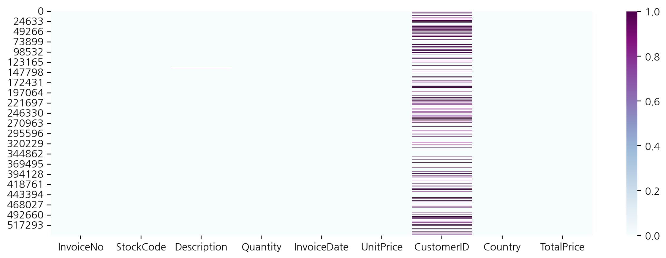
히스토그램 수치변수 시각화
df.hist(figsize=(10, 5), bins=100);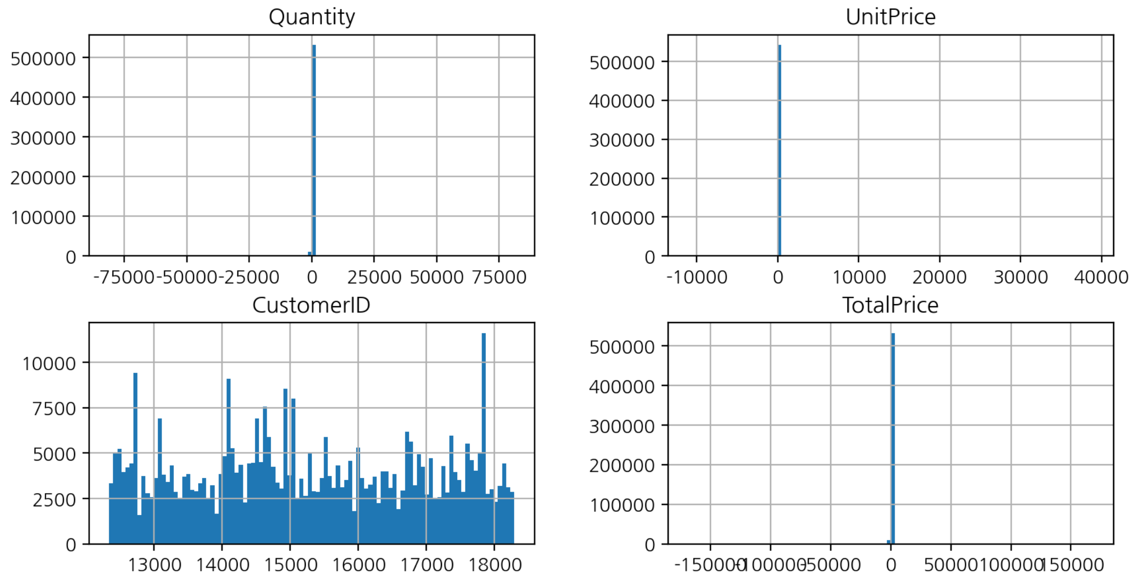
- 1에 가까운 부분에 값이 쏠려있다.
- Quantity, UnitPrice 에 이상치가 있다 ➡️ 범위가 넓게 잡혀있음
전체 주문금액 파생변수
- 수량 * 금액으로 전체 금액 계산
df["TotalPrice"] = df["Quantity"]*df["UnitPrice"]
df.head()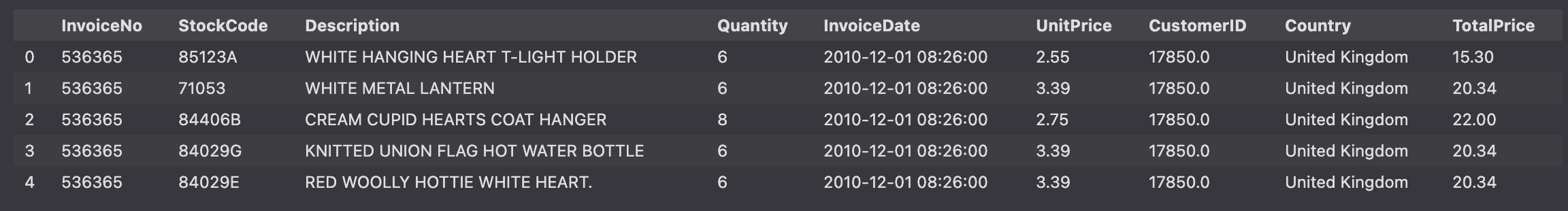
회원 - 비회원 구매
- CustomerID 결측치인 값에 대한 Country값을 가져와 빈도수 구하기
df.loc[df["CustomerID"].isnull(), "Country"].value_counts()
>>>>
United Kingdom    133600
EIRE                 711
Hong Kong            288
Unspecified          202
Switzerland          125
France                66
Israel                47
Portugal              39
Bahrain                2
Name: Country, dtype: int64- CustomerID 결측치가 아닌 값에 대한 Country값을 가져와 빈도수 구하기
df.loc[df["CustomerID"].notnull(), "Country"].value_counts()
>>>>
United Kingdom          361878
Germany                   9495
France                    8491
EIRE                      7485
Spain                     2533
Netherlands               2371
Belgium                   2069
Switzerland               1877
Portugal                  1480
Australia                 1259
Norway                    1086
Italy                      803
Channel Islands            758
Finland                    695
Cyprus                     622
Sweden                     462
Austria                    401
Denmark                    389
Japan                      358
Poland                     341
USA                        291
Israel                     250
Unspecified                244
Singapore                  229
Iceland                    182
Canada                     151
Greece                     146
Malta                      127
United Arab Emirates        68
European Community          61
RSA                         58
Lebanon                     45
Lithuania                   35
Brazil                      32
Czech Republic              30
Bahrain                     17
Saudi Arabia                10
Name: Country, dtype: int64
매출액 상위 국가
- 국가별 매출액의 평균과 합계 구하기
- 상위 10개 추출
df.groupby("Country")["TotalPrice"].agg(['mean',
'sum']).nlargest(10, 'sum').style.format("{:,.0f}")
>>>>
					mean	sum
Country
United Kingdom		17		8,187,806
Netherlands			120		284,662
EIRE				32		263,277
Germany				23		221,698
France				23		197,404
Australia			109		137,077
Switzerland			28		56,385
Spain				22		54,775
Belgium				20		40,911
Sweden				79		36,596
상품
- 판매 빈도가 높은 상품
- 상품 판매 빈도, 판매 총 수량, 총 매출액
stock_sale = df.groupby(['StockCode').agg({"InvoiceNO": "count",
											"Quantity": "sum",
                                            "TotalPrice": "sum",
                                            }).nlargest(10, "InvoiceNO")

stock_sale
>>>>
         	InvoiceNo  Quantity  TotalPrice
StockCode
85123A          2313     38830    97894.50
22423           2203     12980   164762.19
85099B          2159     47363    92356.03
47566           1727     18022    98302.98
20725           1639     18979    35187.31
84879           1502     36221    58959.73
22720           1477      7286    37413.44
22197           1476     56450    50987.47
21212           1385     36039    21059.72
20727 1350 12112 22219.01- 판매 상위 데이터의 Description 구하기
stock_desc = df.loc[df['StockCode'].isin(stock_sale.index),
				["StockCode", "Description"]].drop_duplicates(
                "StockCode", keep='first').set_index("StockCode")
stock_desc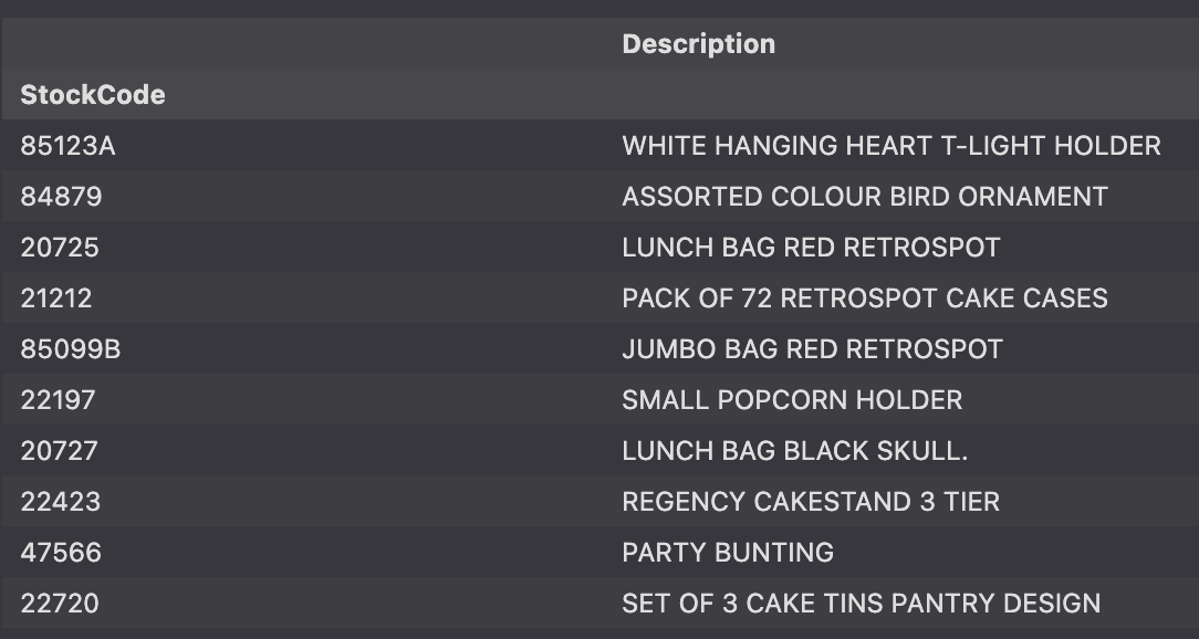
- 판매 상위 데이터에 Description 추가
stock_sale['Desc'] = stock_desc
stock_sale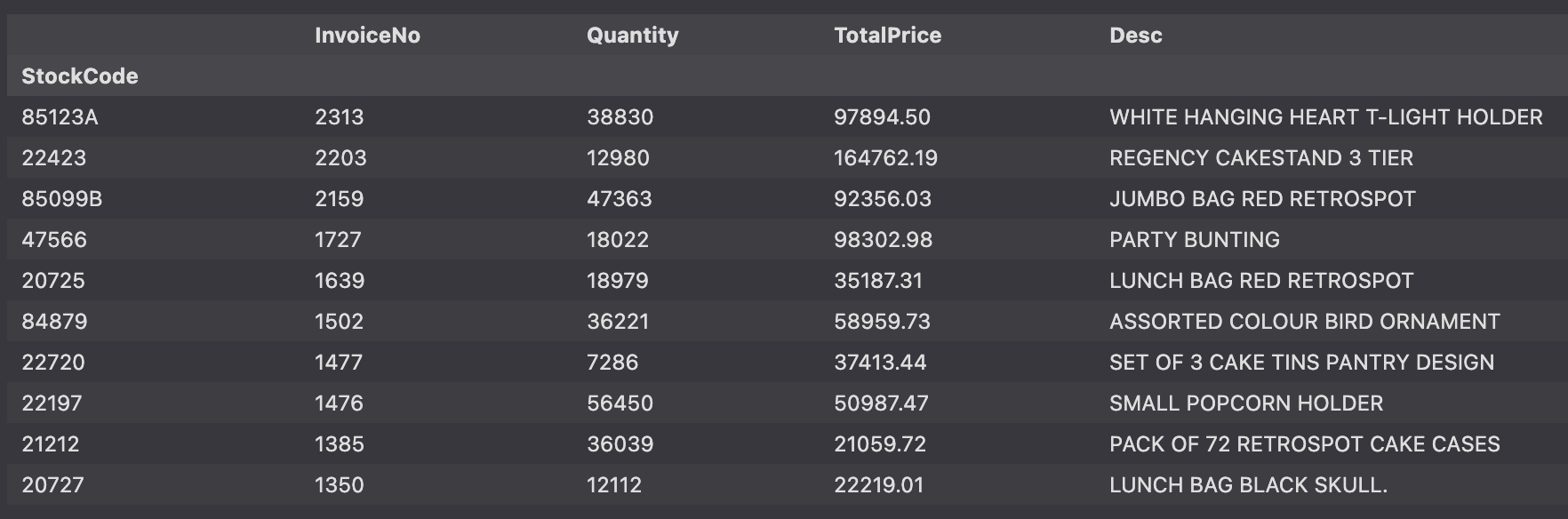
구매 취소 비율
df[df["Quantity"] < 0].head(2)
- 고객별 구매 취소 비율을 찾기 위해 Cancel 컬럼 생성
- Quantity가 0보다 작다면 True, 0보다 크다면 False 값으로 Cancel 컬럼 생성
df["Cancel"] = df["Quantity"] < 0
df.head()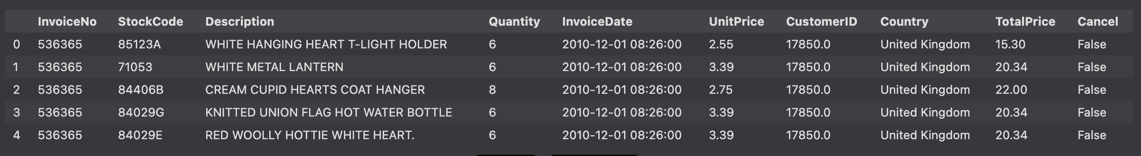
df.groupby("CustomerID")["Cancel"].mean()
>>>>
CustomerID
12346.0    0.500000
12347.0    0.000000
12348.0    0.000000
12349.0    0.000000
12350.0    0.000000
             ...
18280.0    0.000000
18281.0    0.000000
18282.0    0.076923
18283.0    0.000000
18287.0    0.000000
고객별 구매취소 비율
df.groupby("CustomerID")["Cancel"].value_counts(normalize=True)
>>>>
CustomerID  Cancel
12346.0     False     0.500000
            True      0.500000
12347.0     False     1.000000
12348.0     False     1.000000
12349.0     False     1.000000
                        ...
18281.0     False     1.000000
18282.0     False     0.923077
            True      0.076923
18283.0     False     1.000000
18287.0     False     1.000000
고객별 구매 취소 비율 상위 CustomerID 10개
df.groupby("CustomerID")["Cancel"].value_counts().unstack().nlargest(10, False)
>>>>
Cancel       False  True
CustomerID
17841.0     7847.0  136.0
14911.0     5677.0  226.0
14096.0     5111.0   17.0
12748.0     4596.0   46.0
14606.0     2700.0   82.0
15311.0     2379.0  112.0
14646.0     2080.0    5.0
13089.0     1818.0   39.0
13263.0     1677.0    NaN
14298.0     1637.0    3.0
제품별 구매 취소 비율
cancel_stock = df.groupby(['StockCode']).agg({"InvoiceNo":"count",
											"Cancel": "mean"})
cancel_stock.nlargest(10, "InvoiceNo")
>>>>
           InvoiceNo    Cancel
StockCode
85123A          2313  0.018591
22423           2203  0.083522
85099B          2159  0.020380
47566           1727  0.011581
20725           1639  0.026846
84879           1502  0.008655
22720           1477  0.051456
22197           1476  0.033875
21212           1385  0.010830
20727           1350  0.016296
국가별 구매 취소 비율
cancel_country = df.groupby("Country").agg({"InvoiceNo": "count",
											"Cancel": "mean"})
cancel_country.nlargest(20, "Cancel")
>>>>
                  InvoiceNo    Cancel
Country
USA                       291  0.384880
Czech Republic             30  0.166667
Malta                     127  0.118110
Japan                     358  0.103352
Saudi Arabia               10  0.100000
Australia                1259  0.058777
Italy                     803  0.056040
Bahrain                    19  0.052632
Germany                  9495  0.047709
EIRE                     8196  0.036847
Poland                    341  0.032258
Singapore                 229  0.030568
Sweden                    462  0.023810
Denmark                   389  0.023136
Spain                    2533  0.018950
United Kingdom         495478  0.018552
Belgium                  2069  0.018366
Switzerland              2002  0.017483
France                   8557  0.017413
European Community         61  0.016393
날짜와 시간
df["InvoiceDate"] = pd.to_datetime(df["InvoiceDate"])

df["InvoiceYear"] = df["InvoiceDate"].dt.year
df["InvoiceMonth"] = df["InvoiceDate"].dt.month
df["InvoiceDay"] = df["InvoiceDate"].dt.day
df["InvoiceDow"] = df["InvoiceDate"].dt.dayofweek
df.head(1)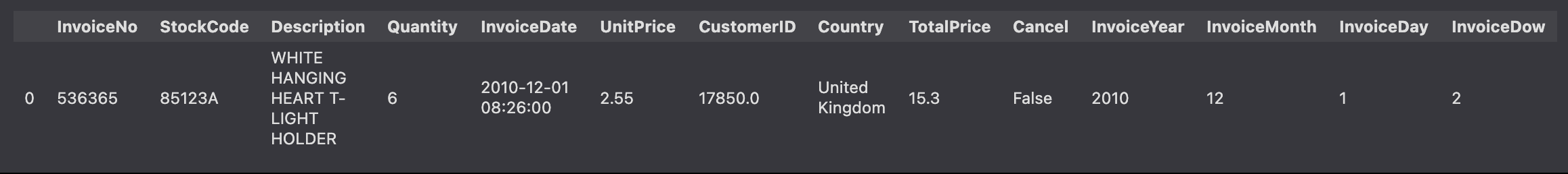
년, 월 따로 생성
df['InvoiceYM'] = df['InvoiceDate'].astype(str).str[:7]
df.head()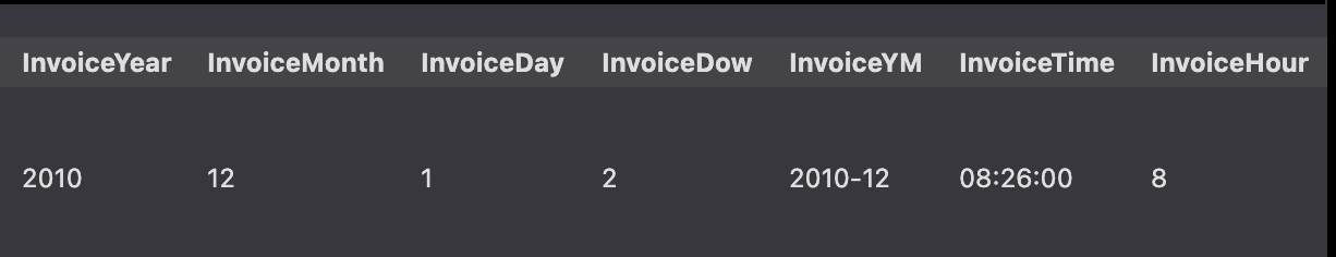
time, hour 파생변수 생성
df["InvoiceTime"] = df["InvoiceDate"].dt.time
df["InvoiceHour"] = df["InvoiceDate"].dt.hour
df.head(1)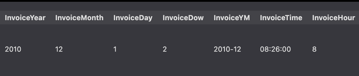
시각화
- 연도별 구매 빈도수 시각화
sns.countplot(data=df, x='InvoiceYear')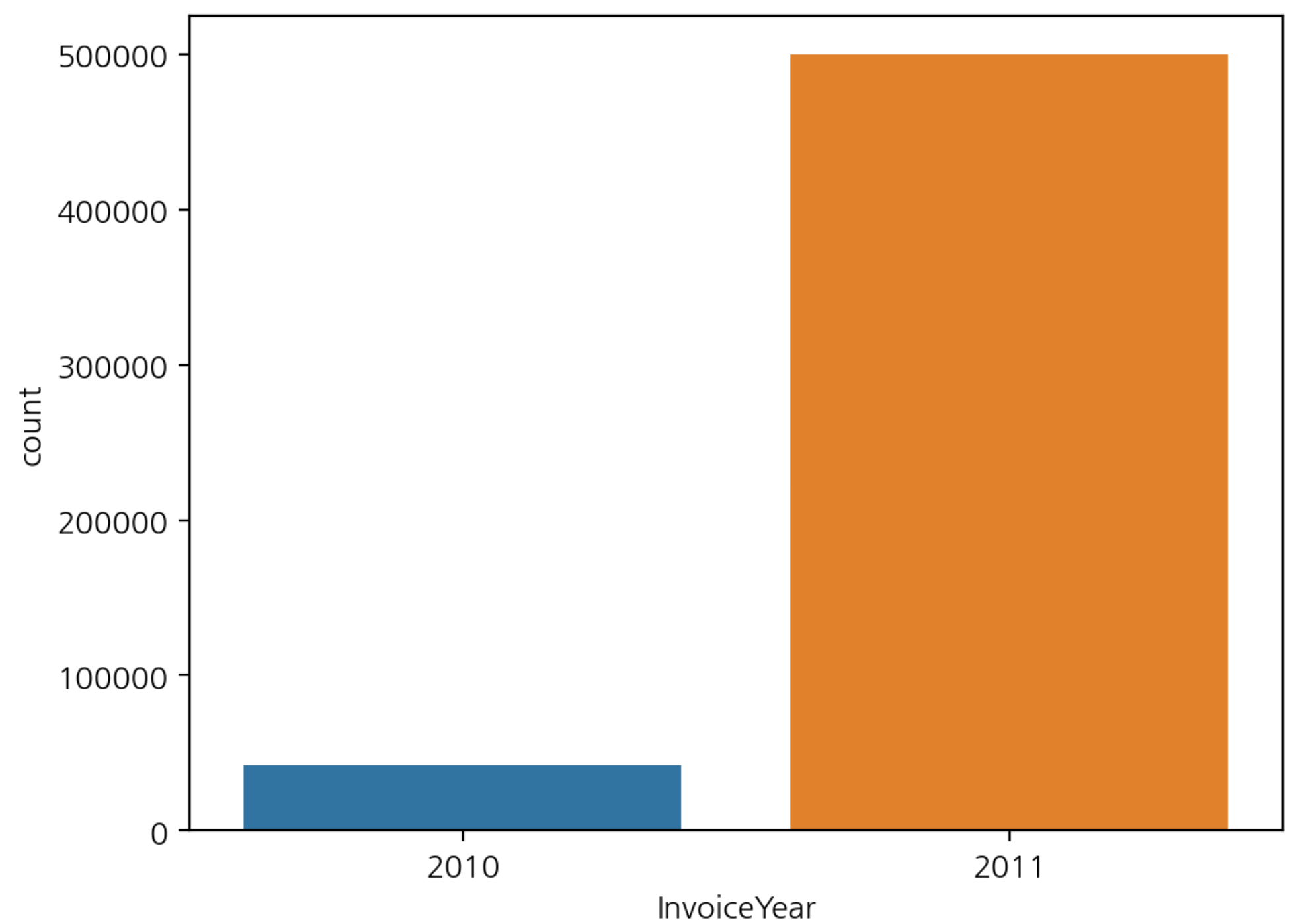
- 월별 구매 빈도수 시각화
sns.countplot(data=df, x='InvoiceMonth')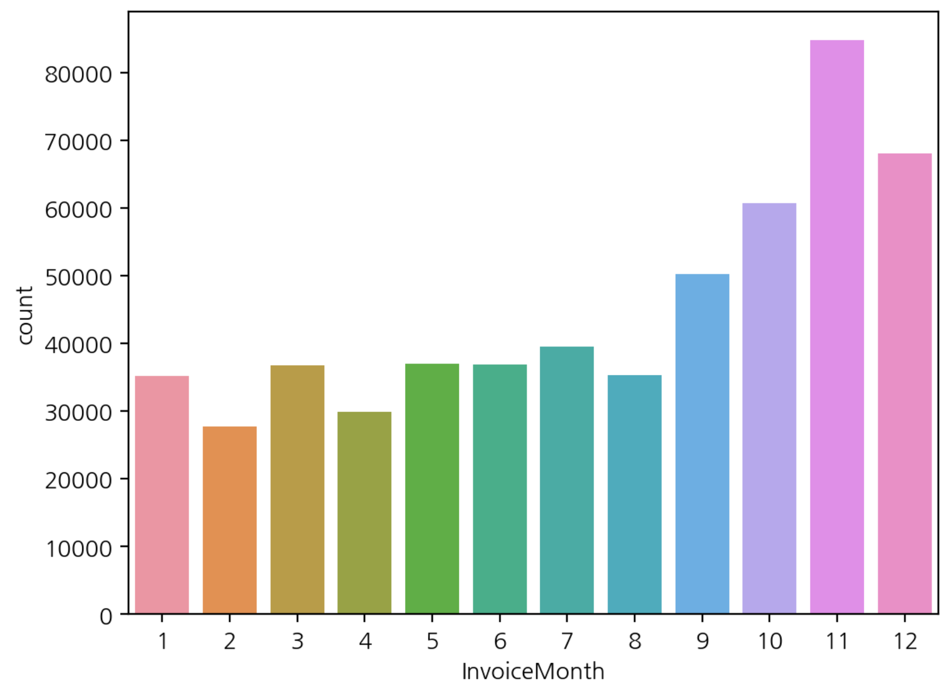
- 연도-월별 구매 빈도수 시각화
plt.figure(figsize=(12, 4))
sns.countplot(data=df, x='InvoiceYM')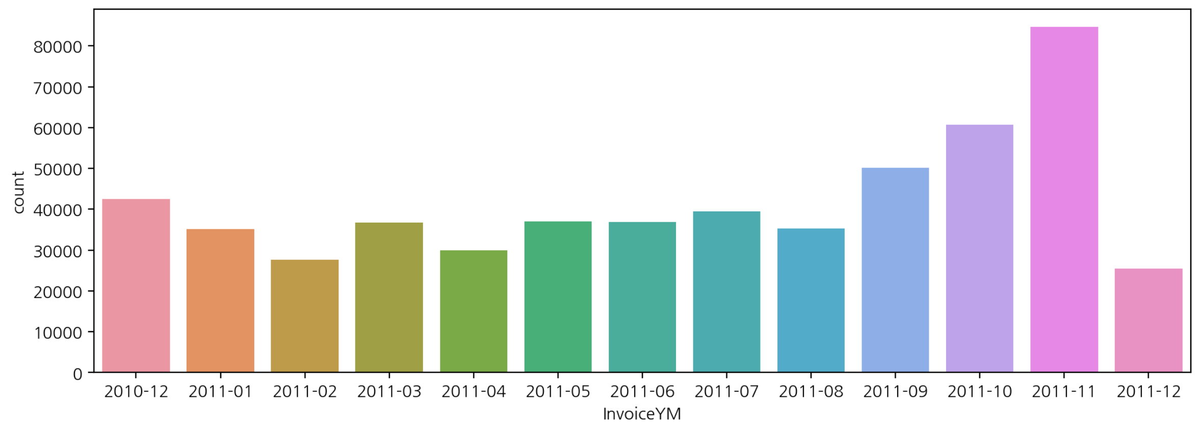
- 요일별 빈도수
sns.countplot(data=df, x='InvoiceDow')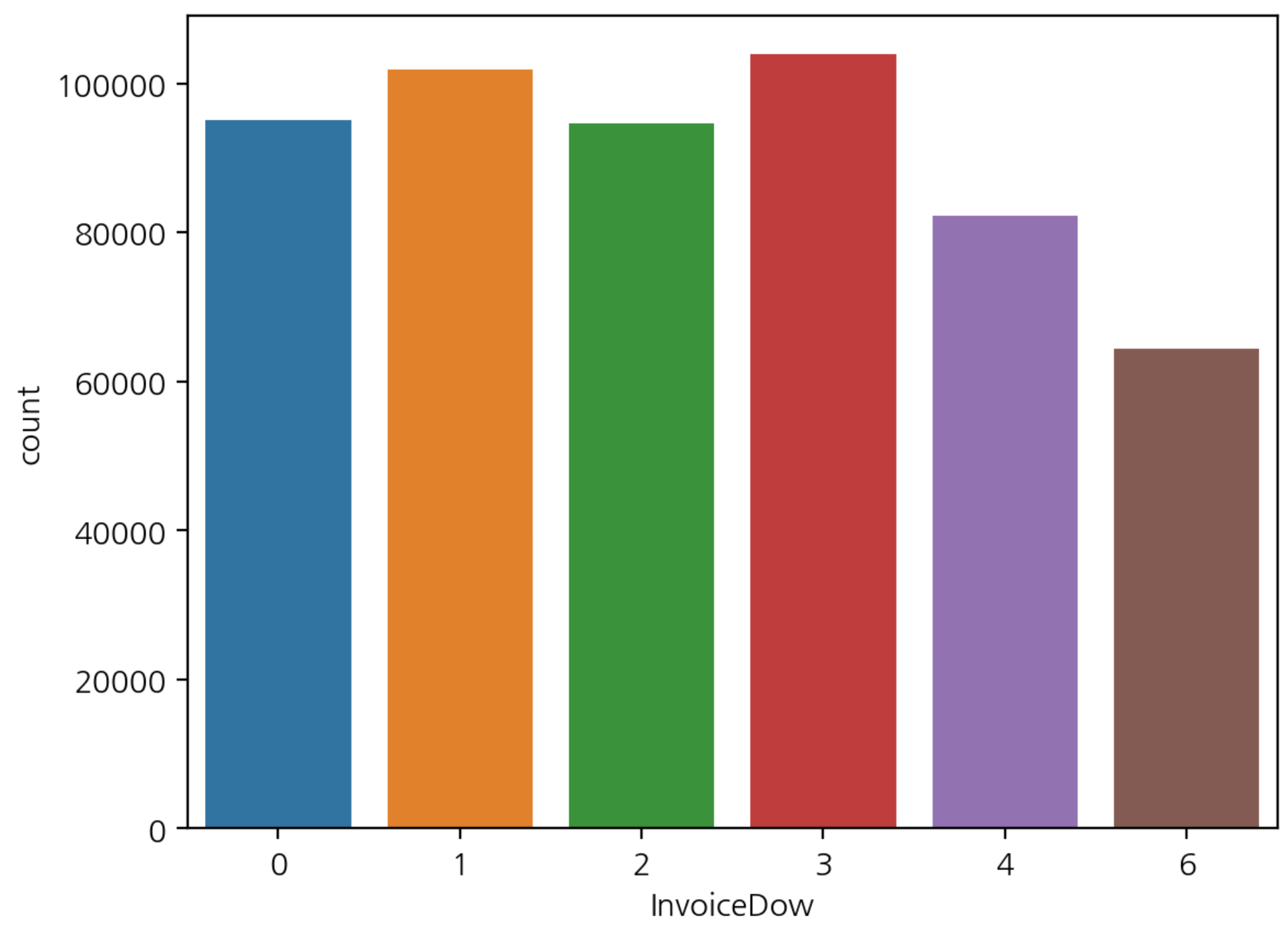
- 요일별 구매와 취소 빈도수 시각화
sns.countplot(data=df, x='InvoiceDow', hue='Cancel')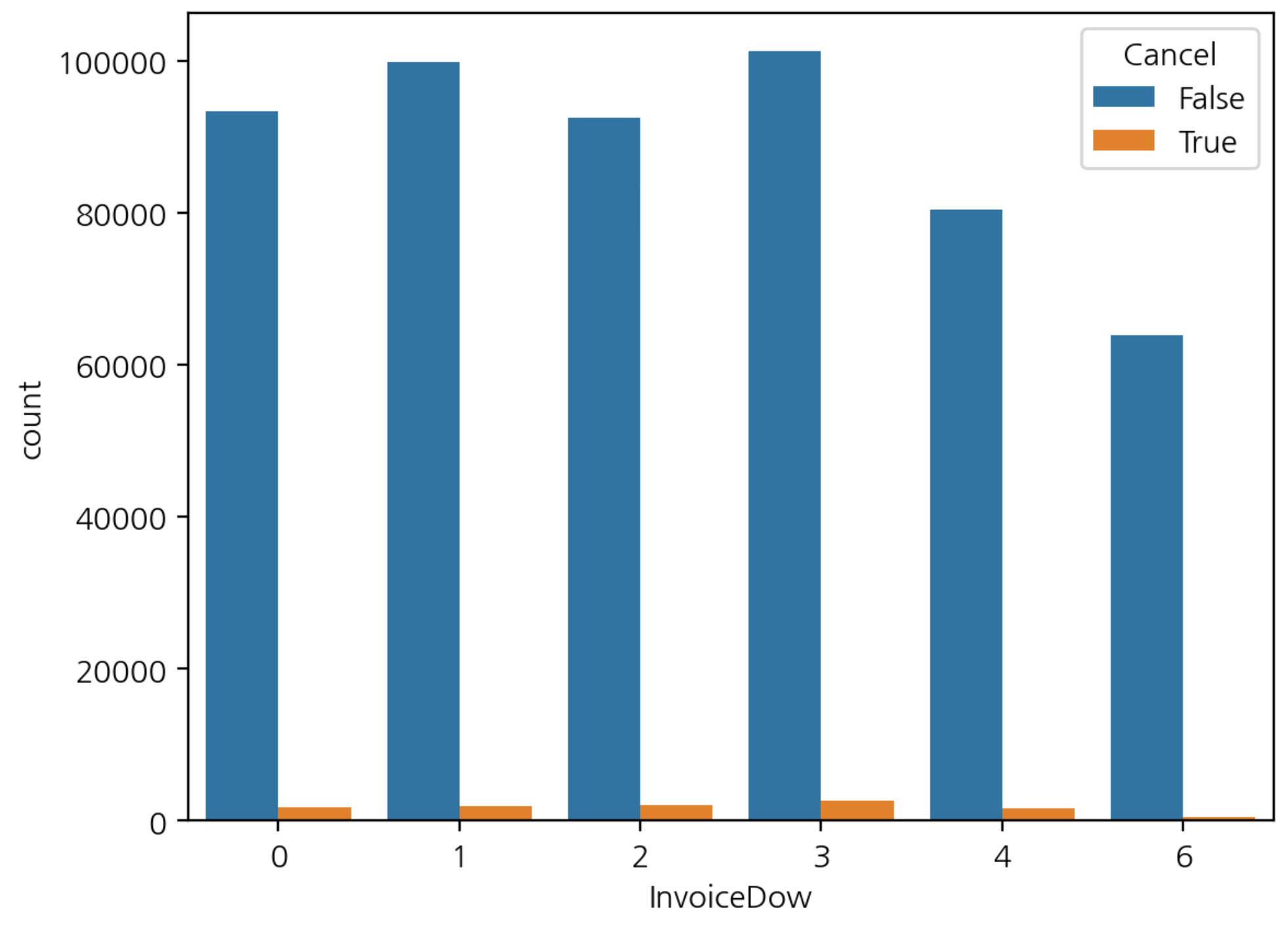
- 요일별 구매 취소 빈도수 시각화
plt.title("요일별 구매 취소")
sns.countplot(data=df[df["Cancel"] == True], x='InvoiceDow')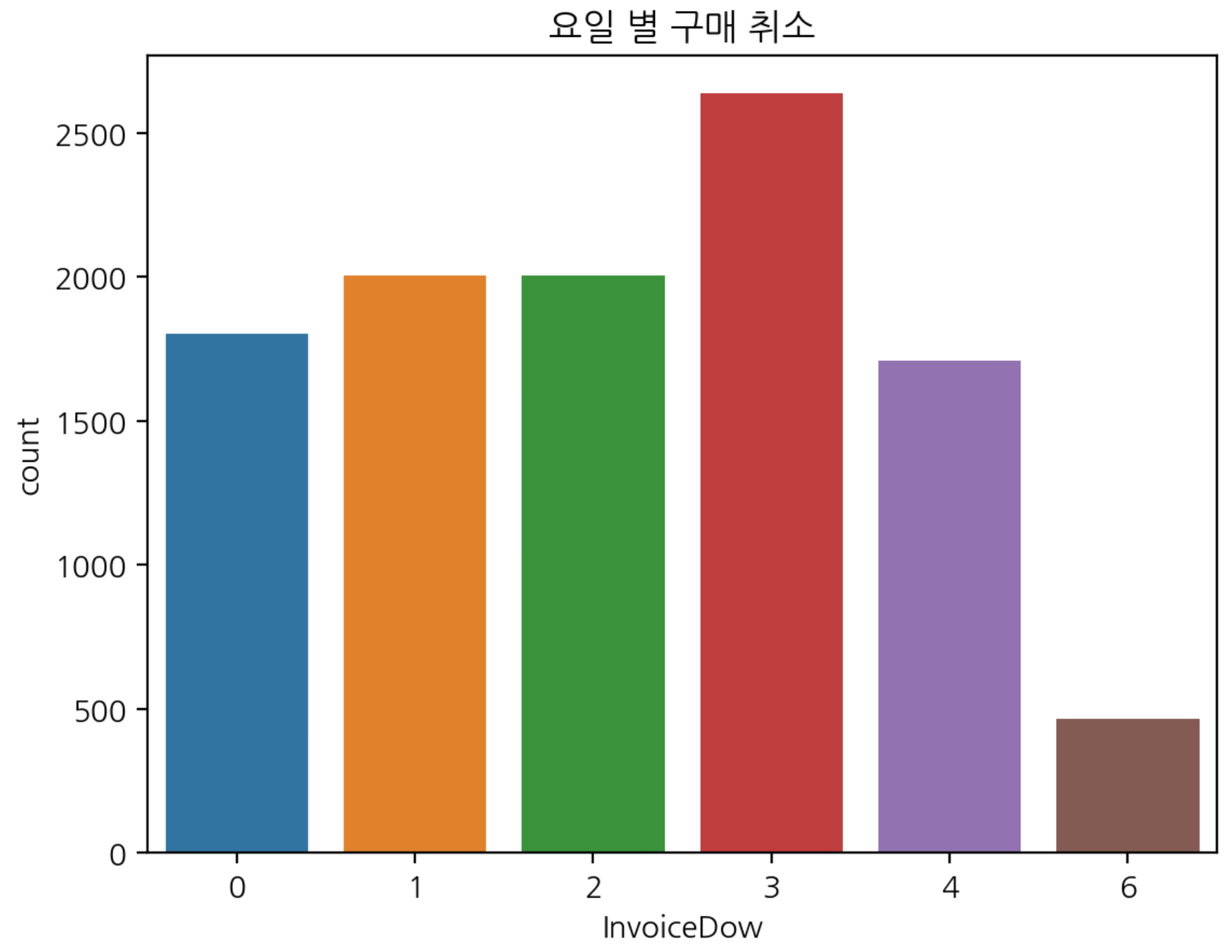
요일 문자열 생성
day_name = [w for w in "월화수목금토일"]

# 데이터를 보면 토요일이 없음
day_name.remove("토")- 요일별 구매 빈도수 구하기
dow_count = df['InvoiceDow'].value_counts().sort_index()
dow_count.index = day_name
dow_count.plot.bar(rot=0, figsize=(7, 3))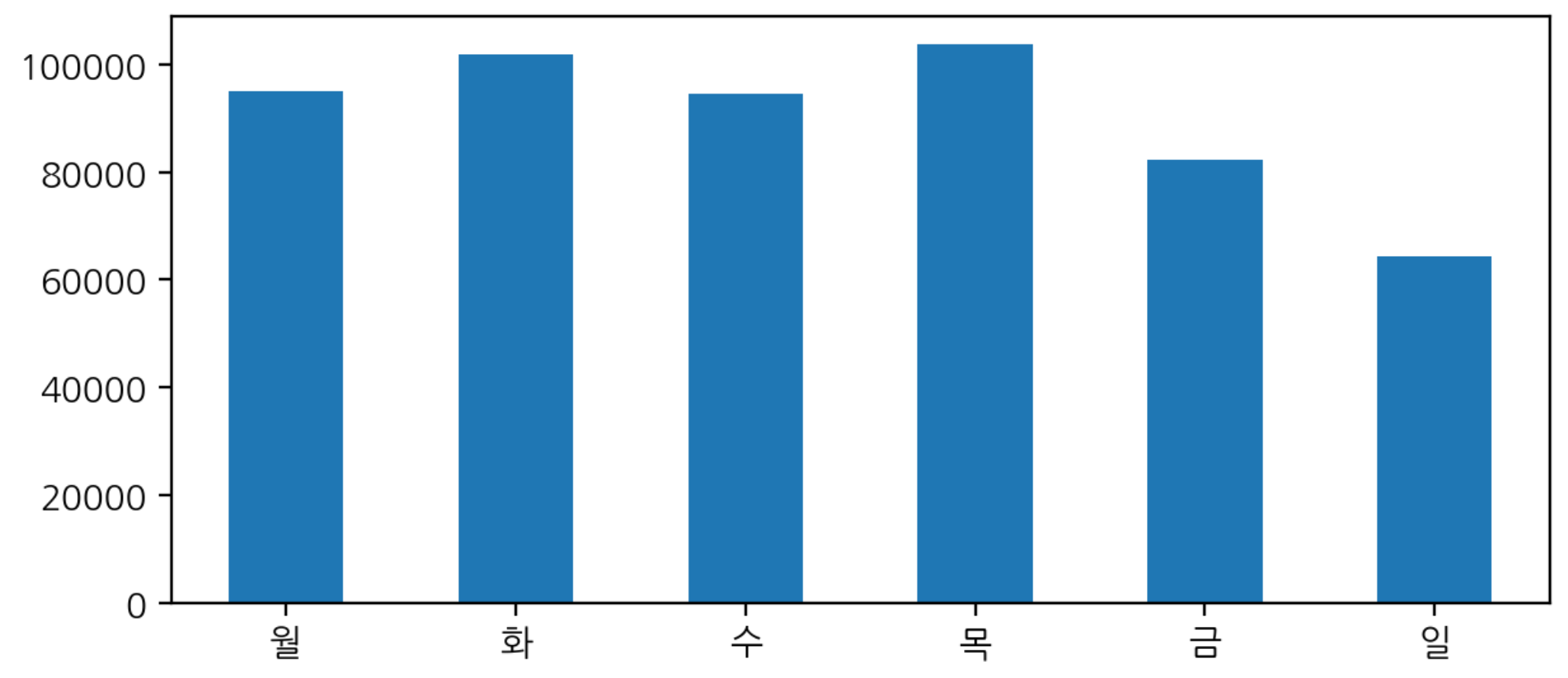
- 시간대 구매 빈도수 시각화
plt.figure(figsize=(12, 4))
sns.countplot(data=df, x='InvoiceHour')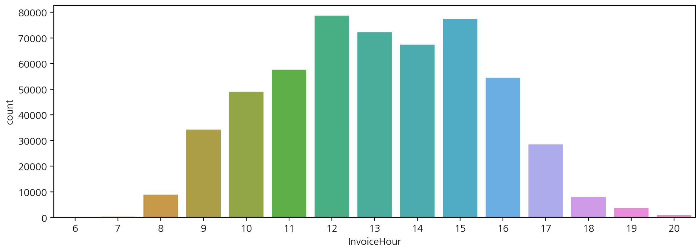
- pointplot을 이용한 시간대 구매 빈도수
plt.figure(figsize=(12, 4))
sns.pointplot(data=df, x="InvoiceHour", y='TotalPrice',
				estimator='count', errorbar=None)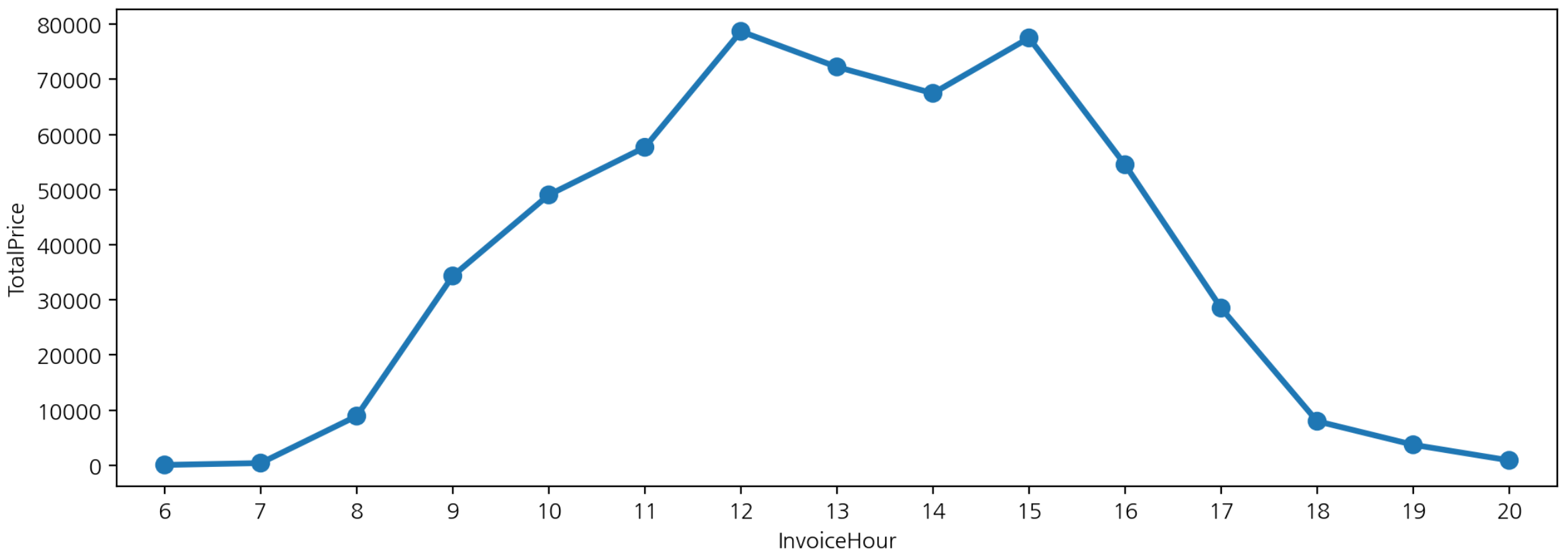
시간-요일별 빈도수
- 시간별, 요일별로 crosstab을 통해 구매 빈도수 구하기
hour_dow = pd.crosstab(index=df['InvoiceHour'], columns=df['InvoiceDow'])
hour_dow.index = day_name
hour_dow
>>>>
               월      화      수      목      금      일
InvoiceHour
6                0      0      0     41      0      0
7               61     65     59     64    134      0
8             1641   1751   1826   1834   1857      0
9             7497   6440   5186   8060   7119     30
10            8872   9125   7904   9321  10215   3600
11            8926  10052   9973   8369   9589  10765
12           11801  14327  14527  13485  10942  13627
13           12756  12619  11901  12428  10488  12067
14           11502  11656  11006  11518  11737  10052
15           13977  16017  16510  11830   9043  10142
16            9529  11924  10768  11765   6438   4092
17            8136   5746   4849   5257   4521      0
18             413   2086     23   5439     13      0
19               0      0     15   3601     89      0
20               0      0     18    845      8      0
시간-요일별 구매 주문 빈도수 시각화
hour_dow.style.background_gradient(cmap='PuBuGn_r').format("{:,}")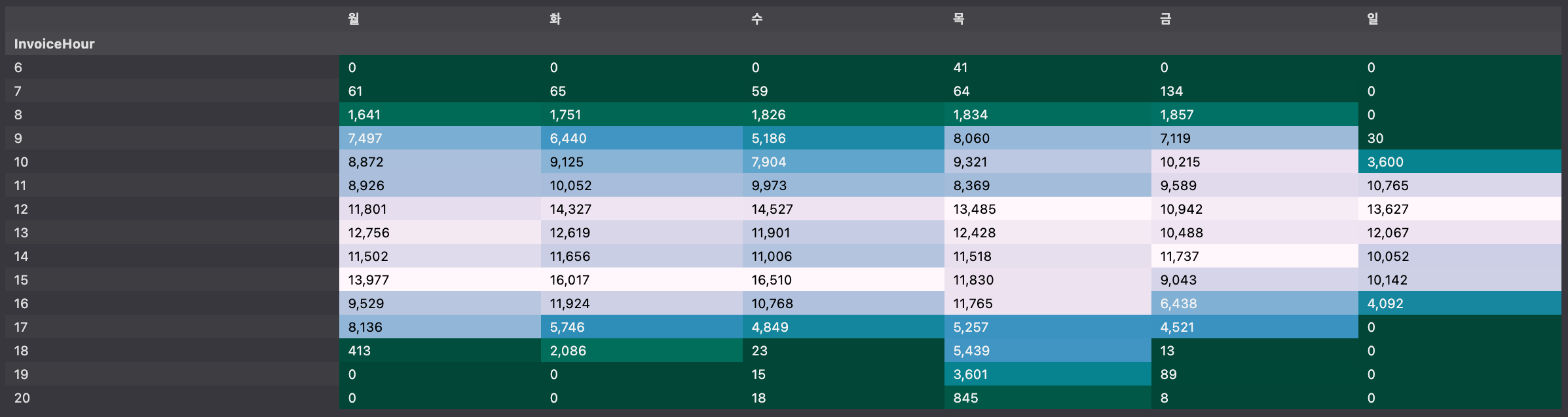
- pandas 의 background_gradient() => 변수마다 성질이 다를 때, 각 변수별로 스케일값을 표현합니다.
- seaborn 의 heatmap() => 같은 성질의 변수를 비교할 때, 전체 수치데이터로 스케일값을 표현합니다.
- heatmap 표현
sns.heatmap(hour_dow, cmap='BuPu', annot=True, fmt=',.0f')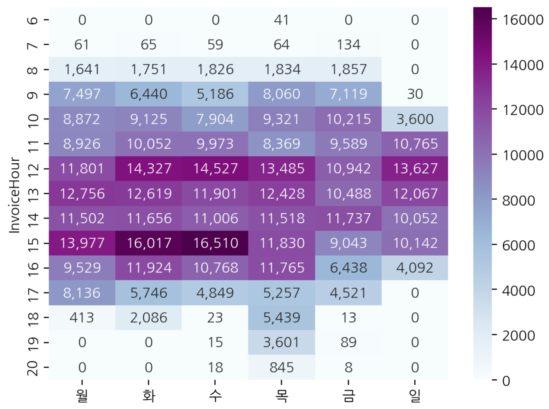
- plot.area 시각화
hour_dow.plot.area(figsize=(12, 3))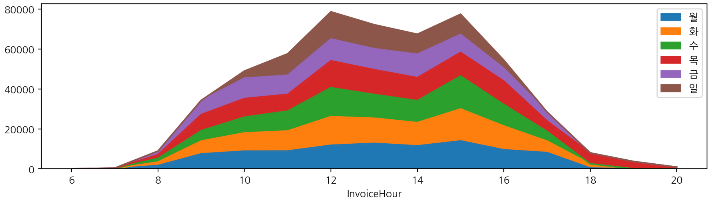
- 시간별 요일별 구매주문 subplot을 통해 요일별 시각화
hour_dow.plot.area(figsize=(12, 5), subplots=True);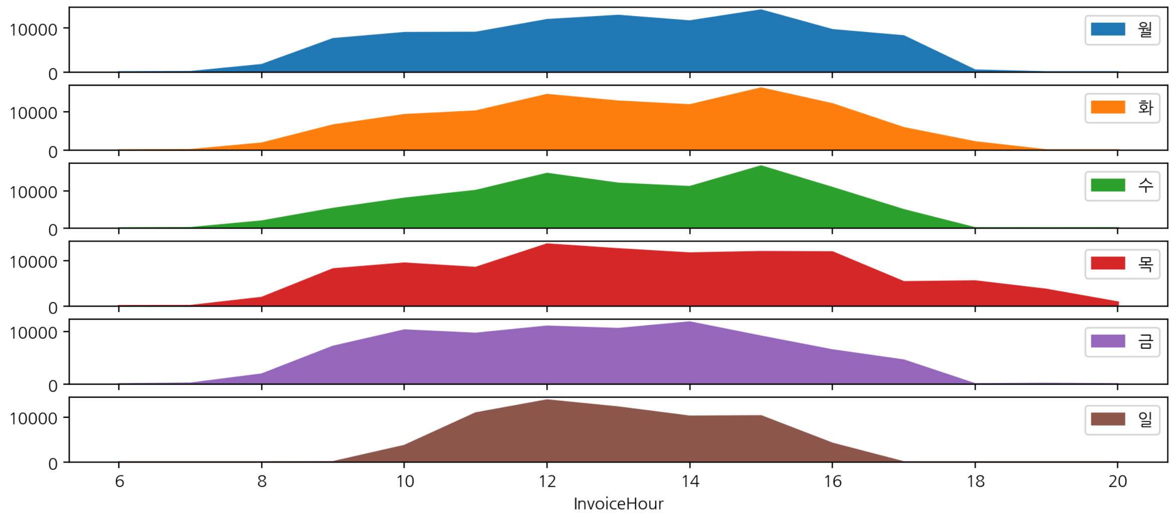
고객ID 없는 주문, 취소 주문 제외
- 취소와 취소에 대한 본 주문건 제외
- 고객 ID가 없는 건 제외
- CustomerID가 있고(notnull) "Quantity, UnitPrice" 가 0보다 큰 데이터 가져오기
df_valid = df[df['CustomerID'].notnull() & (df["Quantity"] > 0) & (df["UnitPrice"] > 0)].copy()

df.shape, df_valid.shape
>>>>
((541909, 17), (397884, 17))

# 중복 데이터 제거
df_valid = df_valid.drop_duplicates()
df_valid.shape
>>>>
(392692, 17)
고객 (ARPPU)
ARPU : Average Revenue Per User
- 가입한 서비스에 대해 가입자 1명이 특정 기간 동안 지출한 평균 금액
- ARPU = 매출 / 중복을 제외한 순수 활동 사용자 수
ARPPU : Average Revenue Per Paying User
- 지불 유저 1명당 한 달에 결제하는 평균 금액을 산정한 수치
# ARPPU : CustomerID 를 사용할 때는 count가 아닌 nunique 사용 -> 중복을 고려하지 않는다
arppu = df_valid.groupby("InvoiceYM").agg({"TotalPrice":"sum", "CustomerID":"nunique"})
arppu.columns = ['sale_sum', 'customer_count']
arppu["ARPPU"] = arppu['sale_sum'] / arppu['customer_count']
arppu.style.format("{:,.0f}")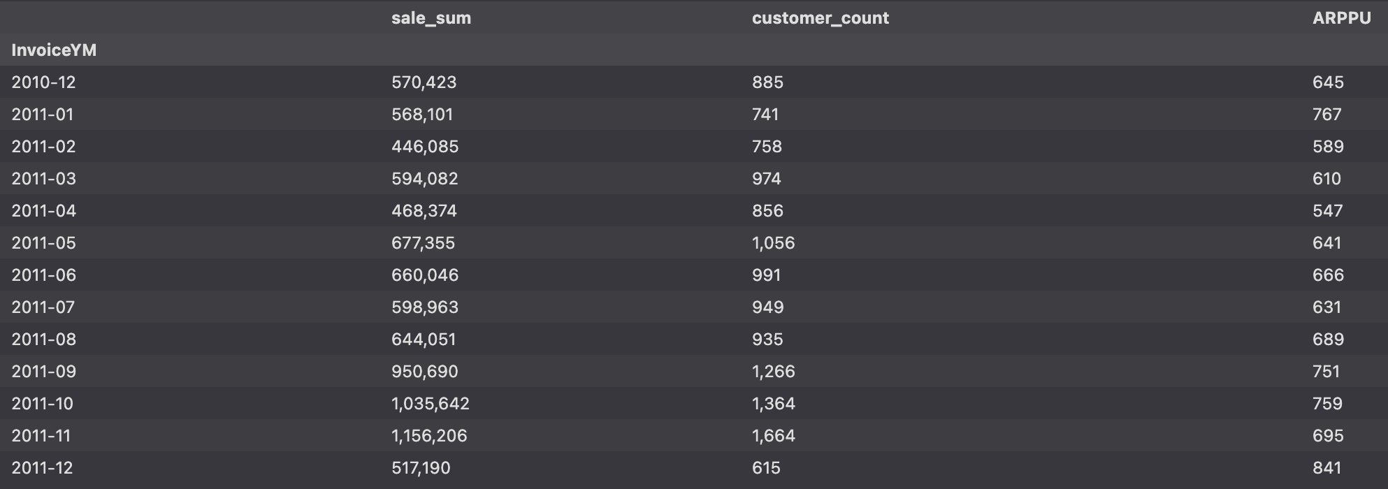
시각화
arppu['ARPPU'].plot(figsize=(10, 3), title="Monthly ARPPU")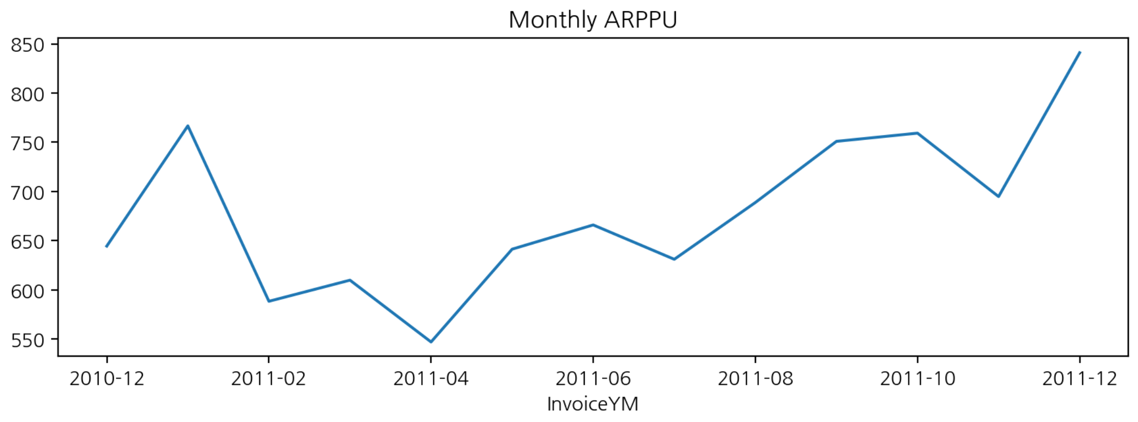
- df_valid(유효고객, 유효주문)내 고객별 (CustomerID) 구매 (InvoiceNo) 빈도수 구하기
- 고객별 구매 빈도수, 평균 구매 금액, 총 구매 금액
cust_agg = df_valid.groupby(['CustomerID']).agg({"InvoiceNo":['nunique', 'count'],
											'TotalPrice':['mean', 'sum']})

cust_agg.columns = ['nunique', 'count', 'mean', 'sum']
cust_agg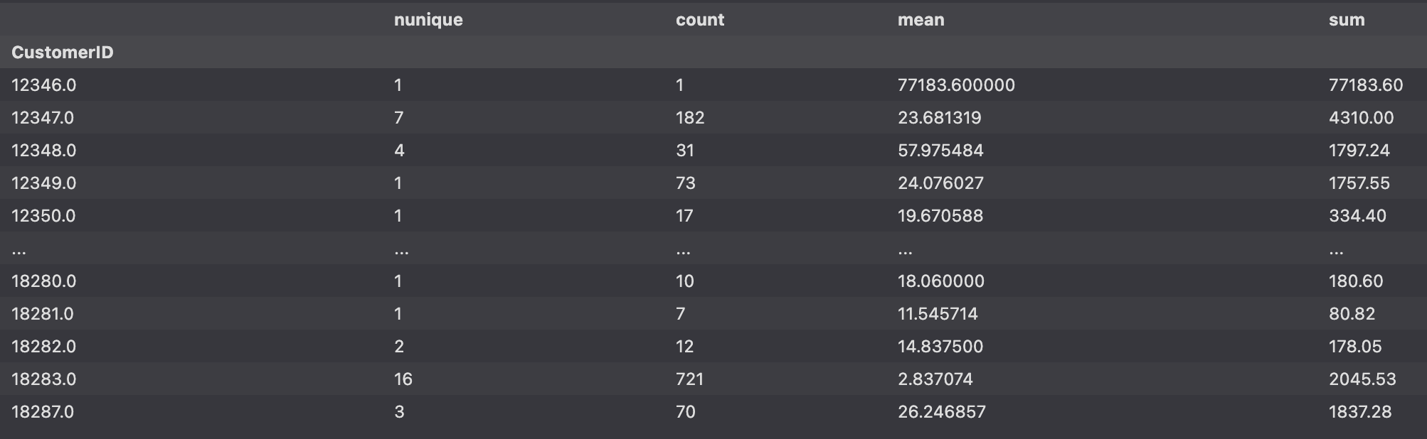
MAU (Monthly Active User)
- InvoiceYM 으로 그룹화하여 CustomerID의 유일값의 개수를 구한다.
- MAU 기준은 로그인 수 or 구매 수
mau = df_valid.groupby('InvoiceYM')['CustomerID'].agg('nunique')
mau.plot.bar(figsize=(10, 3), rot=30, title="MAU(Monthly Active User)")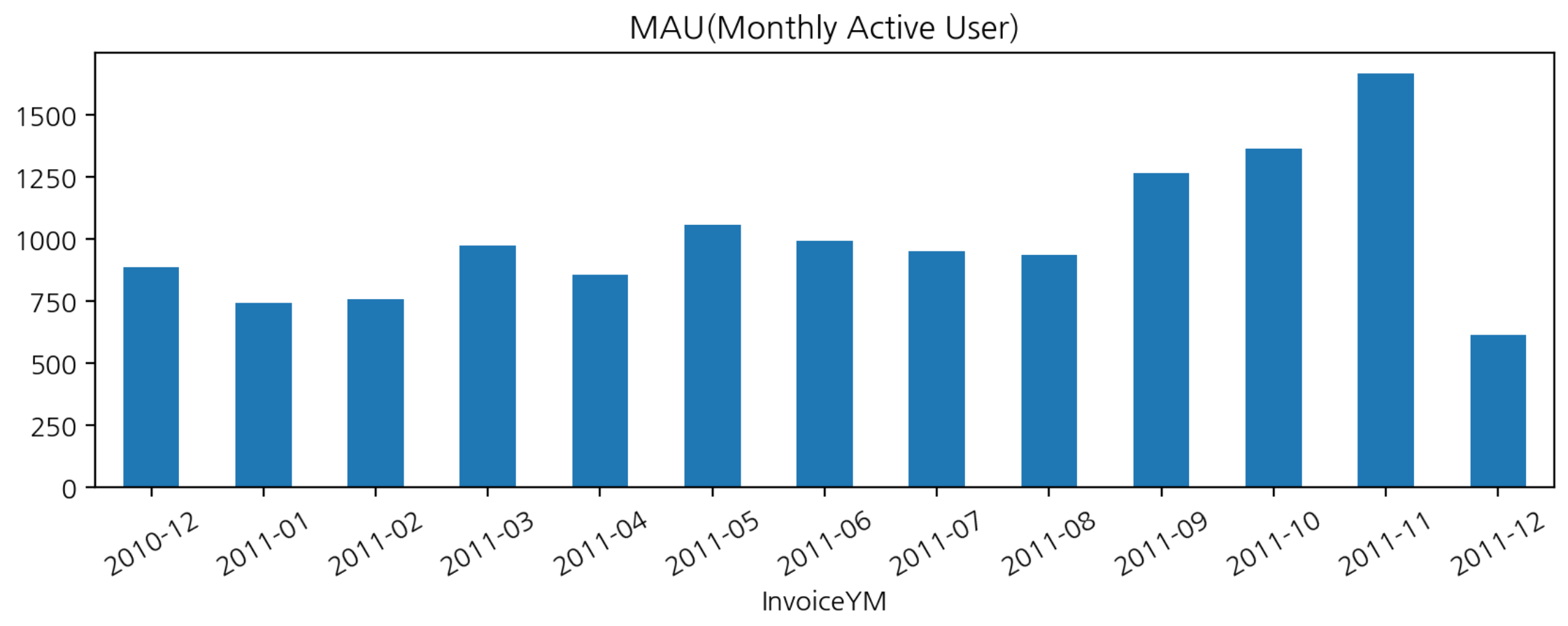
중복을 제외한 제품 종류 수, 고객 수, 총 금액
- 월별, 주문건 중복을 제외한 주문제품의 종류 수, 고객의 수, 총 주문금액 구하기
df_valid.groupby("InvoiceYM").agg({"InvoiceNo" : "count",
                             "StockCode": "nunique",
                             "CustomerID": "nunique",
                             "UnitPrice" : "sum",
                             "Quantity" : "sum",
                             "TotalPrice" : "sum"})
>>>>
          InvoiceNo  StockCode  CustomerID   UnitPrice  Quantity   TotalPrice
InvoiceYM
2010-12        25670       2411         885   80679.600    311048   570422.730
2011-01        20988       2121         741   66234.650    348473   568101.310
2011-02        19706       2124         758   62619.480    265027   446084.920
2011-03        26870       2234         974   87864.790    347582   594081.760
2011-04        22433       2217         856   78543.481    291366   468374.331
2011-05        28073       2219        1056  101500.910    372864   677355.150
2011-06        26926       2339         991   84602.660    363014   660046.050
2011-07        26580       2351         949   75454.521    367360   598962.901
2011-08        26790       2356         935   78877.090    397373   644051.040
2011-09        39669       2545        1266  118160.322    543652   950690.202
2011-10        48793       2622        1364  164084.090    591543  1035642.450
2011-11        63168       2695        1664  182340.090    665923  1156205.610
2011-12        17026       2173         615   46559.700    286777   517190.440
Retention
- 해당 고객의 첫 구매월을 찾는다.
- 첫 구매월과 해당 구매 시점의 월 차이를 구한다.
- 첫 구매한 달로부터 몇 달 만에 구매한 것인지 구한다.
월단위 데이터 전처리
df_valid['InvoiceDate1'] = pd.to_datetime(df_valid["InvoiceYM"])
df_valid['InvoiceDate1'].head()
>>>>
0   2010-12-01
1   2010-12-01
2   2010-12-01
3   2010-12-01
4   2010-12-01
-> 일자를 '1'로 통일한 이유는 월별 잔존율을 구하기 위해서 (월 단위)
df_valid[["InvoiceDate", "InvoiceDate1"]].sample(5)
>>>>
               InvoiceDate InvoiceDate1
431356 2011-10-31 14:48:00   2011-10-01
7755   2010-12-05 11:40:00   2010-12-01
150305 2011-04-08 11:54:00   2011-04-01
285985 2011-08-01 13:31:00   2011-08-01
91562 2011-02-16 10:47:00 2011-02-01- 최초 구매월(InvoiceDateMin)에 InvoiceDate1의 최솟값을 할당
- 일자가 '1'로 통일되어 있어 최근 구매일 - 최초 구매일 로 첫 구매 후 몇 달만에 구매인지 확인
df_valid["InvoiceDateMin"] = df_valid.groupby('CustomerID')['InvoiceDate1'].transform('min')
df_valid["InvoiceDateMin"]
>>>>
0        2010-12-01
1        2010-12-01
2        2010-12-01
3        2010-12-01
4        2010-12-01
            ...
541904   2011-08-01
541905   2011-08-01
541906   2011-08-01
541907   2011-08-01
541908 2011-08-01- InvoiceDateMin : 최초구매월
- InvoiceDate1 : 해당구매월
df_valid[["CustomerID", "InvoiceDate", "InvoiceDateMin", "InvoiceDate1"]].sample(5)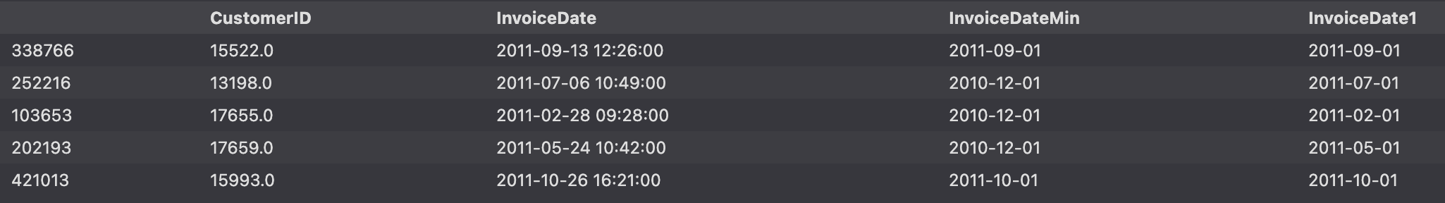
첫 구매일로 부터 몇 달째 구매인가?
- 연도별 차이, 월별 차이 구한다
- 해당 구매일 - 최초 구매일
year_diff = df_valid['InvoiceDate1'].dt.year - df_valid['InvoiceDateMin'].dt.year
year_diff
month_diff = df_valid['InvoiceDate1'].dt.month - df_valid['InvoiceDateMin'].dt.month
month_diff- " 연도차이 * 12개월 + 월차이 + 1 "로 첫 구매 후 몇달 후 구매인지 알 수 있도록 CohortIndex 변수를 생성합니다.
- 2010-12-01부터 2011-12-01의 데이터를 기반으로 진행되어 CohortIndex 변수의 최소값은 1이며, 최대값 13입니다.
df_valid["CohortIndex"] = (year_diff * 12) + month_diff + 1
df_valid[['CustomerID', 'InvoiceDate1', 'InvoiceDateMin', 'CohortIndex']].sample(5)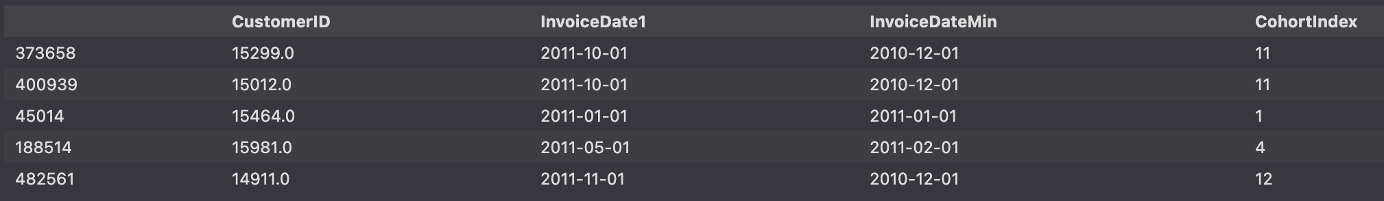
코호트 월별 빈도수
- 월별 잔존 구매에 대한 빈도수 구하기
df_valid['CohortIndex'].value_counts().sort_index()
>>>>
1     116857
2      27516
3      26727
4      26993
5      25165
6      26673
7      23462
8      23298
9      22751
10     22968
11     20098
12     23011
13 7173- 시각화
plt.figure(figsize=(12, 4))
sns.countplot(data=df_valid, x='CohortIndex')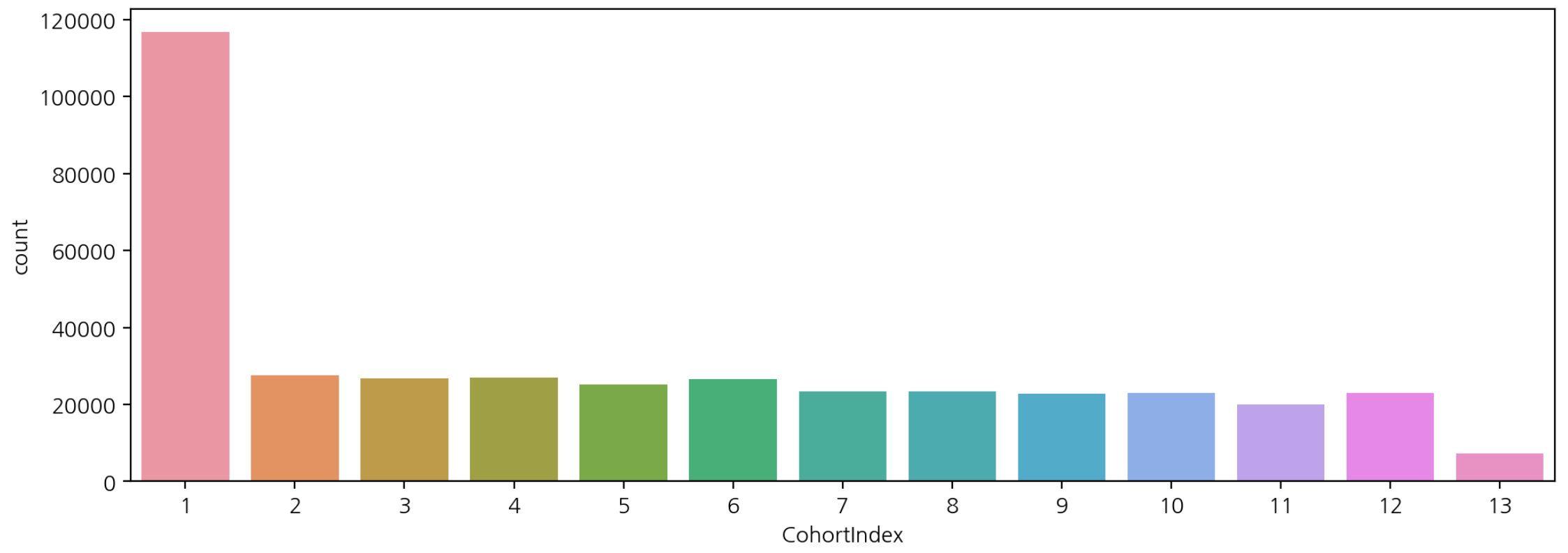
➡️ 첫 달에만 구매하고 다음달 부터 구매하지 않는 사람이 많다.
➡️ 마케팅비 많이 쏟아서 고객을 유치했지만 유지가 잘 되지 않는 것으로 보여진다.
➡️ 휴면 고객을 위한 이벤트, 쿠폰 등이 적절한 시점에 있으면 도움이 되겠다는 계획을 세워볼 수 있다.
잔존 빈도 구하기
cohort_count = df_valid.groupby(['InvoiceDateMin', 'CohortIndex'])['CustomerID'].nunique().unstack()
cohort_count.index = cohort_count.index.astype(str)
cohort_count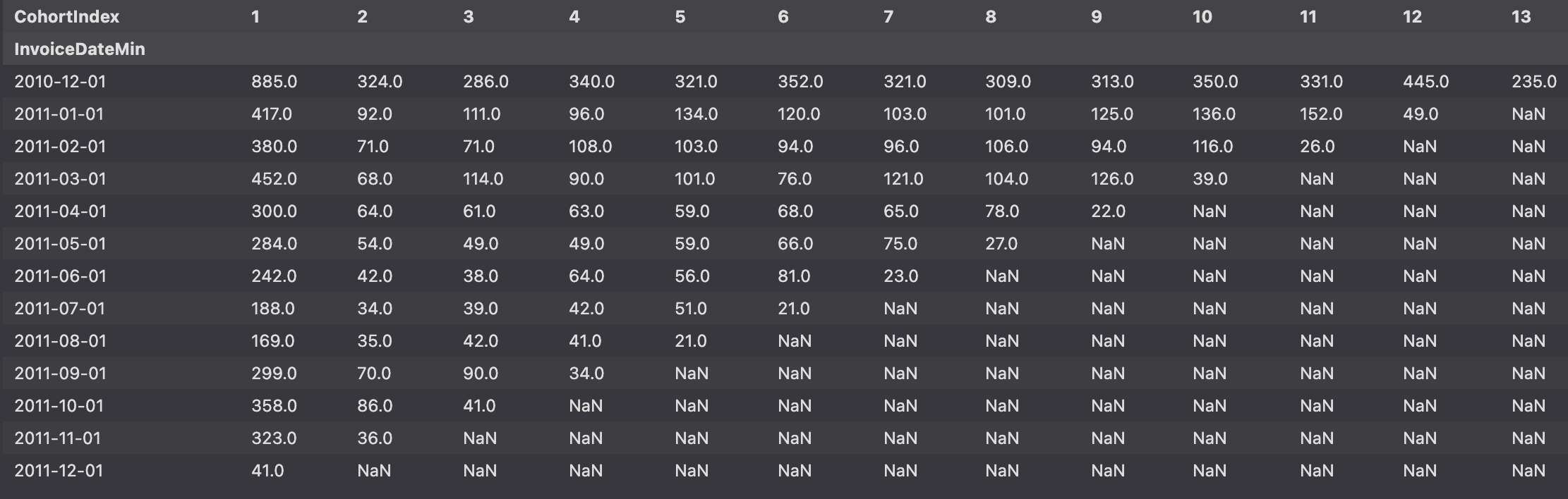
잔존수 시각화
plt.figure(figsize=(12, 8))
sns.heatmap(cohort_count, annot=True, fmt=".0f", cmap="BuPu")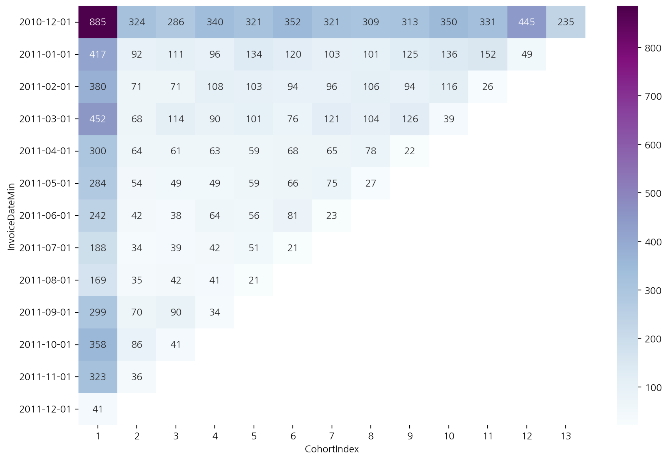
월별 신규 유입 고객 수
- Acquisition
cohort_count[1].plot.bar(figsize=(16, 3), title="월별 신규 유입 수", rot=0)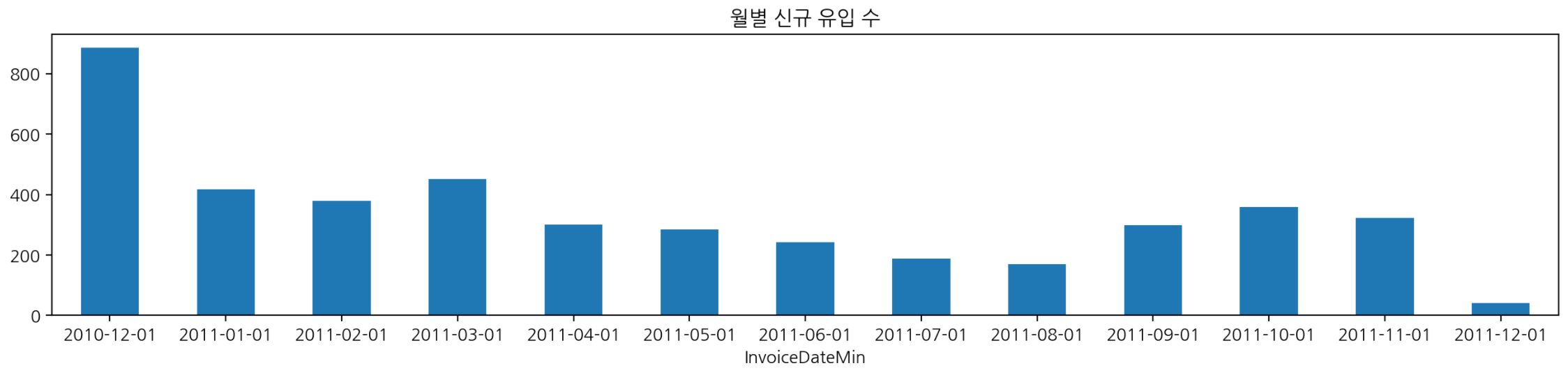
잔존율
- 가입한 달을 1로 나누면 잔존율 구할 수 있음
- div 를 통해 구하며 axis=0 으로 설정하면 첫 달을 기준으로 나머지 달을 나누게 된다.
cohort_norm = cohort_count.div(cohort_count[1], axis=0)
cohort_norm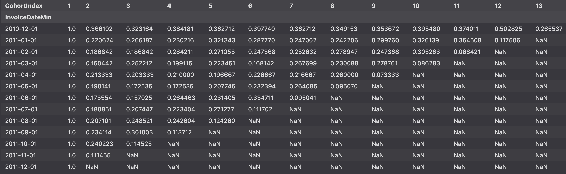
잔존율 heatmap
plt.figure(figsize=(12, 8))
sns.heatmap(cohort_norm, cmap="BuPu", annot=True, fmt=".2f")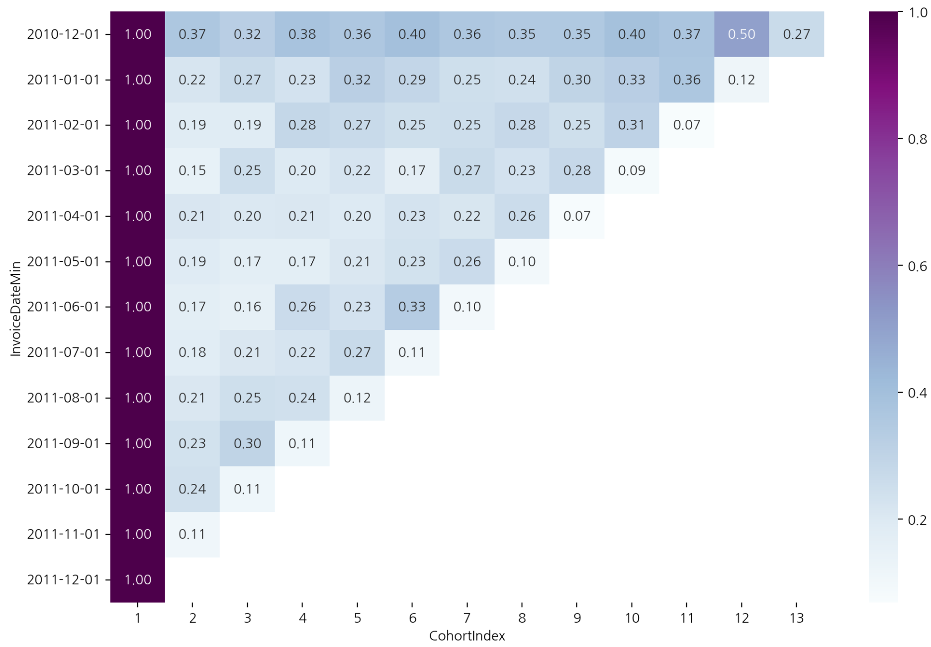
- 코호트 분석에서 시간 단위로 묶어서 보는 분석 중 하나가 리텐션 분석
- 같은 달에 첫 구매한 사람들이 같은 집단으로 묶였기 때문에 시간 단위 코호트 분석이 된다.

Ⓓ🅰️🅣🄰 ♡♥︎