📍 RNN
: Recurrent Neural Network
- RNN이 기존 신경망과의 차이점 : 결과값을 출력층 방향으로 보내면서, 다시 은닉층 노드의 다음 계산의 입력으로 보내는 특징
- 다양한 길이의 입력 시퀀스를 처리할 수 있는 인공신경망
- 텍스트 분류나 기계 번역과 같은 다양한 자연어 처리에 대표적으로 사용되는 인공신경망
- 타임스텝(timestep) : 입력 시퀀스의 길이(input_length)라고도 표현
- 순환네트워크에서는 은닉층이 입력층과 이전 타임스텝의 은닉층으로부터 정보를 받음
- 인접한 타임스텝의 저보가 은닉층에 흐르기 때문에 이전 이벤트를 기억 가능(신경망 내부의 메모리를 활용)
❗️등장 배경
- 기존 모델의 한계점 : 전부 은닉층에서 활성화 함수를 지난 값은 오직 출력층 방향으로만 향함 (한 방향)
- 시퀀스 데이터 (순서가 있는 자료로 시계열 자료나 텍스트 자료)를 기존 모델인 NN, CNN으로는 처리 성능이 낮았음
- 가중치가 데이터의 처리되는 순서와 상관없이 업데이트 되기 때문에 이전에 본 샘플을 기억할 수 없음
- 피드 포워드 신경망 (은닉층에서 활성화 함수를 지난 값은 오직 출력층 방향으로만) 은 입력의 길이가 고정
❗️유형
- One to one : 가장 기본적인 모델
- One to many : 하나의 이미지를 문장으로 표현
- Many to one : 단어의 시퀀스에 대해서 하나의 출력을 하는 구조로 감정 분류, 주가 등락을 통한 회사의 파산 여부 분류 등
- 영화 리뷰를 통해 긍정 또는 부정으로 감정 분류
- 주가 등락을 통한 회사의 파산 여부 분류
❗️용어
- cell : RNN의 은닉층에서 활성화 함수를 통해 결과를 내보내는 역할을 하는 노드
- memory cell : 이전의 값을 기억하는 일종의 메모리 역할을 수행하는 셀 (전체, RNNcell)
- hidden state : 은닉층의 메모리 셀에서 나온 값이 출력층 방향 또는 다음 시점의 자신 (다음 메모리 셀) 에게 보내는 상태
RNN의 역전파 ❓
: BackPropagation Through Time (BPTT)
- 기울기는 오차의 변화에 대한 가중치의 변화이기 때문에 모델에 맞는 역전파 방법으로 기울기를 찾아야 성능을 높일 수 있음
- 다른 신경망과 마찬가지로 RNN 역시 경사 하강법 (Gradient Descent)과 오차 역전파를 이용해 학습
- 정확하게는 시간의 흐름에 따른 작업을 하기 때문에 역전파를 확장한 BPTT를 사용해 학습
- RNN은 기존 신경망의 역전파와 달리 타임스텝별로 네트워크를 펼친 다음, 역전파 알고리즘을 사용
- 타임스텝의 역방향으로 역전파를 통해 가중치 비율을 조정하여 오차 감소를 진행
- 일정 시간 동안 오차 값들을 합한 값을 역전파함으로써 현재 시간의 오차를 과거 시간의 상태까지 역전파
RNN의 학습(Overview)
- RNN은 이전 작업을 현재 작업과 연결할 수 있다는 장점
- 인공 신경망과 다르게 RNN은 순환 구조이므로 은닉층의 데이터를 저장하며 펼쳐진 형태로 순환구조로 확률값을 계산
진행 방향 〽️
1️⃣ tf.keras.Sequential
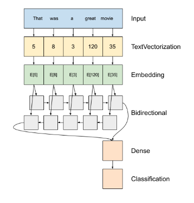
2️⃣ 첫 번째 층은 encoder 토큰 인덱스의 시퀀스에 텍스트를 반환
3️⃣ 인코더 후 임베딩 레이어
- 텍스트 인코더 만들기 : encoder.adapt() 층의 어휘를 설정 (fit_transform 과 유사)
- 임베딩 레이어는 단어당 하나의 벡터를 저장. 호출되면 단어 인덱스 시퀀스를 벡터 시퀀스로 변환
- 이러한 벡터는 훈련이 가능. (충분한 데이터에 대한) 훈련 후 유사한 의미를 가진 단어는 종종 유사한 벡터를 가진다.
4️⃣ RNN은 요소를 반복하여 시퀀스 입력을 처리한다. RNN은 한 타임 스텝의 출력을 다음 타입 스텝의 입력으로 전달
- tf.keras.layers.Bidirectional 래퍼는 또한 RNN 층으로 사용될 수 있음. 이것이 RNN 레이어를 통해 입력을 앞뒤로 전파한 다음 최종 출력을 연결
5️⃣ RNN 단일 벡터에 순서를 전환한 후, 두 layers.Dense 분류 출력으로 단일 로짓이 벡터 표현에서 일부 최종 처리 및 변환 함.

model = tf.keras.Sequential([
    encoder,
    tf.keras.layers.Embedding(
        input_dim=len(encoder.get_vocabulary()),
        output_dim=64,
        # Use masking to handle the variable sequence lengths
        mask_zero=True),
    tf.keras.layers.Bidirectional(tf.keras.layers.LSTM(64)),
    tf.keras.layers.Dense(64, activation='relu'),
    tf.keras.layers.Dense(1)
])
word embedding ❓
: 유사한 단어가 유사한 인코딩을 갖는 효율적이고 조밀한 표현을 사용하는 방법을 제공
➡️ 단어를 특정 차원의 벡터로 바꿔 주는 것
- 기계가 이해하기 쉽도록 텍스트를 벡터(숫자배열)로 변환
- 인코딩을 직접 지정할 필요가 없다.
- 부동 소수점의 값을 조밀한 벡터
- 임베딩에 대한 값을 수동으로 지정하는 대신 학습 가능한 매개변수
- 큰 데이터 세트로 작업할 때 9차원, 최대 1024차원의 단어 임베딩을 보는 것이 일반적
- 더 높은 차원의 임베딩은 단어 간의 세분화된 관계를 캡쳐할 수 있지만 더 많은 데이터가 필요
# Embed a 1,000 word vocabulary into 5 dimentions
embedding_layer = tf.keras.layers.Embedding(1000, 5)
✅ 임베딩 레이어를 생성할 때 임베딩의 가중치는 다른 레이어와 마찬가지로 무작위로 초기화 된다.
훈련하는 동안 역전파를 통해 점진적으로 조정된다.
일단 훈련되면 학습된 단어 임베딩은 단어 간의 유사성을 대략적으로 인코딩한다.
📍 해당 TextVectorization은 단어의 맥락을 고려하는 것이 아니라 빈도수에 따른 단어 사전의 위치만 알려준다. 따라서 TextVectorization으로 학습하는 것은 큰 의미가 없다.
✅ 따라서 TextVectorization을 Embedding을 시켜주고 좌표로 표시할 수 있다.
맥락이 비슷하면 좌표에서 거리를 가깝게 옮겨주고 맥락이 반대면 좌표에서 거리를 멀게 설정해준다.
이 거리를 설정하는 과정은 LSTM에서 학습 후 조정해주게 된다.
❗️ Modeling ❗️
📌 SimpleRNN
- 층을 순서대로 쌓아 분류기(classifier)를 만든다.
- 첫 번째 층은 Embedding 층이다. 이 층은 정수로 인코딩 된 단어를 입력 받고 각 단어의 인덱스에 해당하는 임베딩 벡터를 찾는다. 이 벡터는 모델이 훈련되면서 학습된다.
- 기본적으로 RNN 레이어의 출력에는 샘플당 하나의 벡터가 포함된다.
- return_sequences = True 설정하면 RNN 레이어가 각 샘플에 대한 전체 출력 시퀀스도 반환할 수 있다.
📌 LSTM
등장 배경
- RNN의 기울기 소실 : RNN의 구조상 관련 정보와 그 정보를 사용하는 지점 사이의 거리가 멀 경우, 역전파하는 과정이 너무 길어져 기울기 값이 아주 작아져 소실되는 문제가 발생
- 입력의 길이가 길어져도 이전 정보를 더 오래 기억하는 학습 방법의 필요성
- 장단기(Long Short-Term Memory, LSTM)는 순환 신경망 기법의 하나
- 메모리 셀, 입력 게이트, 출력 게이트, 망각 게이트를 이용해 기존 순환 신경망의 기울기 소실 문제를 방지
정의
- LSTM 알고리즘은 Cell State라고 불리는 특징층을 하나 더 넣어 Weight를 계속 기억할 것인지 결정
- 셀 상태 (Cell State)는 정보를 추가하거나, 삭제하는 기능을 담당
-> LSTM은 과거의 데이터를 계속해서 업데이트 - 기존 RNN의 경우, 정보와 정보 사이의 거리가 멀면 초기 Weight 값이 유지되지 않아 학습능력이 저하
- 장점 : 각각의 메모리 컨트롤이 가능
- 단점 : 메모리가 덮어씌워 질 가능성이 있음
📌 GPUs (Gated Recurrent Units)
- LSTM을 변형시킨 알고리즘으로 Gradient Vanishing의 문제 해결
- LSTM은 초기의 Weight가 계속 지속적으로 업데이트되었지만, GPUs는 Update Gate와 Reset Gate를 추가하여 과거의 정보를 어떻게 반여할 것인지 결정 (GPU는 게이트 2개, LSTM은 3개)
- Update Gate : 과거의 상태를 반영하는 Gate
- Reset Gate : 현 시점 정보와 과거 시점 정보의 반영 여부 결정
📝 실습
라이브러리 & 데이터 로드
import numpy as np
import pandas as pd
import matplotlib.pyplot as plt
import seaborn as sns
df = pd.read_csv("https://bit.ly/seoul-120-text-csv")
df.shape
>>>>
(2645, 5)
df.head(2)
- 제목과 내용을 합쳐서 문서라는 파생변수 만든다
df['문서'] = df['제목'] + " " + df['내용']

df['분류'].value_counts()
>>>>
행정        1098
경제         823
복지         217
환경         124
주택도시계획     110
문화관광        96
교통          90
안전          51
건강          23
여성가족        13
Name: 분류, dtype: int64- 일부 상위 분류 데이터만 추출
df = df[df['분류'].isin(['행정', '경제', '복지'])]
df.shape
>>>>
(2138, 6)
문제, 정답값 만들기
label_name = '분류'

X = df['문서']
y = df[label_name]

X.shape, y.shape
>>>>
((2138,), (2138,))
label one-hot 형태
- one-hot-encoding 하는 이유?
: 분류 모델의 출력층을 softmax로 사용하기 위해
📍 softmax 각 클래스의 확류값을 반환하여 각각의 클래스의 합계를 구하면 1이 된다.
y_onehot = pd.get_dummies(y)
y_onehot.head(2)
>>>>
  경제  복지  행정
0   0   1   0
1   1   0   0
train_test_split
from sklearn.model_selection import train_test_split
X_train, X_test, y_train, y_test = train_test_split(X, y_onehot, test_size=0.2, stratify=y_onehot, random_state=42)
X_train.shape, X_test.shape, y_train.shape, y_test.shape
>>>>
((1710,), (428,), (1710, 3), (428, 3))
display(y_train.value_counts(normalize=True))
display(y_test.value_counts(normalize=True))
>>>>
경제 복지 행정
0 0 1 0.513450
1 0 0 0.384795
0 1 0 0.101754
dtype: float64
경제 복지 행정
0 0 1 0.514019
1 0 0 0.385514
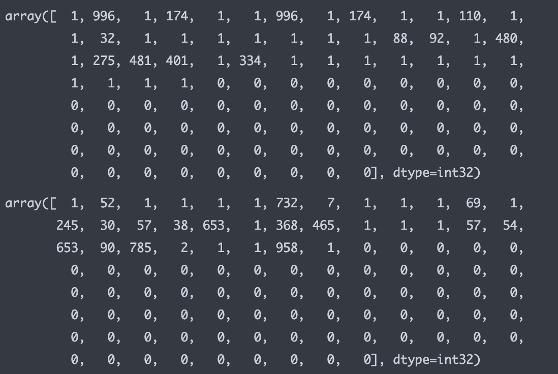
0 1 0 0.100467padding
: 병렬 연산을 위해 여러 문장의 길이를 임의로 동일하게 맞춰주는 작업이 필요
- 문장의 길이가 제각각인 벡터의 크기를 패딩 작업을 통해 나머지 빈 공간을 0으로 채워준다.
from tensorflow.keras.preprocessing.sequence import pad_sequence

max_length = 500
padding_type = 'post'

X_train_sp = pad_sequences(train_sequence, maxlen=max_length, padding=padding_type)
X_test_sp = pad_sequences(test_sequence, maxlen=max_length, padding=padding_type)

X_train_sp.shape, X_test_sp.shape
>>>>
((1710, 500), (428, 500))

display(X_train_sp[0, :100])
display(X_test_sp[0, :100])
>>>>
Modeling
📍 SimpleRNN
from tensorflow.keras import Sequential
from tensorflow.keras.layers import Dense, Embedding, SimpleRNN, GRU, Bidirectional, LSTM, Dropout, BatchNormalization

# embedding_dim : 임베딩 할 벡터의 차원
# vocab_size : 텍스트 데이터의 전체 단어 집합의 크기
# max_length : 패딩의 기준

embadding_dim = 64
n_class = y_train.shape[1]

model = Sequential()
# 입력-임베드 층
model.add(Embedding(input_dim=vocab_size,
					output_dim=embadding_dim,
                    input_length=max_length))
model.add(Bidirectional(SimpleRNN(units=64, return_sequences=True))
model.add(Bidirectional(SimpleRNN(units=64, return_sequences=True))
model.add(SimpleRNN(units=64))

# 출력층
model.add(Dense(units=n_class, activation='softmax'))
model.summary()
>>>>
Model: "sequential_19"
_________________________________________________________________
 Layer (type)                Output Shape              Param #
=================================================================
 embedding_2 (Embedding)     (None, 500, 64)           64000

 bidirectional_12 (Bidirecti  (None, 500, 128)         16512
 onal)

 bidirectional_13 (Bidirecti  (None, 500, 128)         24704
 onal)

 simple_rnn_34 (SimpleRNN)   (None, 64)                12352

 dense_28 (Dense)            (None, 3)                 195

=================================================================
Total params: 117,763
Trainable params: 117,763
Non-trainable params: 0
compile
model.compile(optimizer='adam',
				loss='categorical_crossentropy',
                metrics=['accuracy'])
학습
from tensorflow.keras.callbacks import EarlyStopping
early_stop = EarlyStopping(monitor='val_loss', patience=5)- validation data 만들고 학습
X_train_val, X_valid, y_train_val, y_valid = train_test_split(
	X_train_sp, y_train, test_size=0.2, random_state=42, stratify=y_train)

X_train_val.shape, X_valid.shape, y_train_val.shape, y_valid.shape
>>>>
((1368, 500), (342, 500), (1368, 3), (342, 3))
history = model.fit(X_train_val, y_train_val, validation_data=(X_valid, y_valid),
epochs=100, callbacks=[early_stop])
history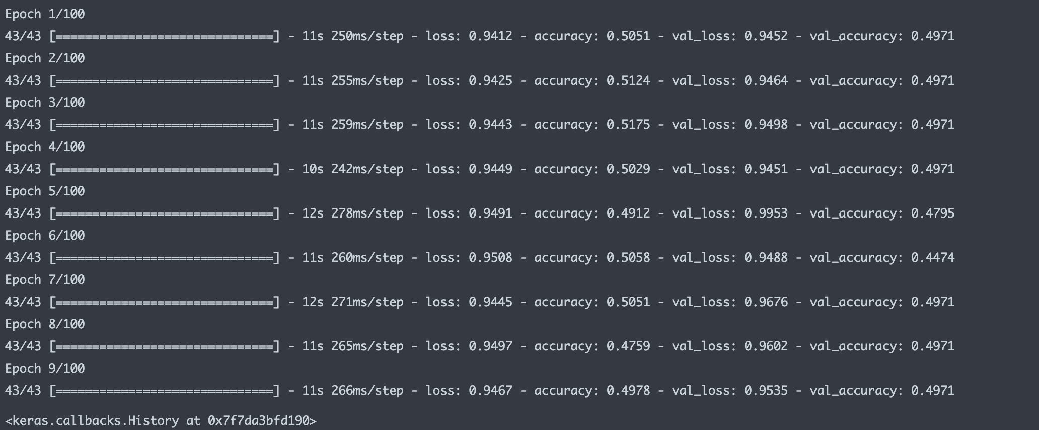
df_hist = pd.DataFrame(history.history)
df_hist
>>>>
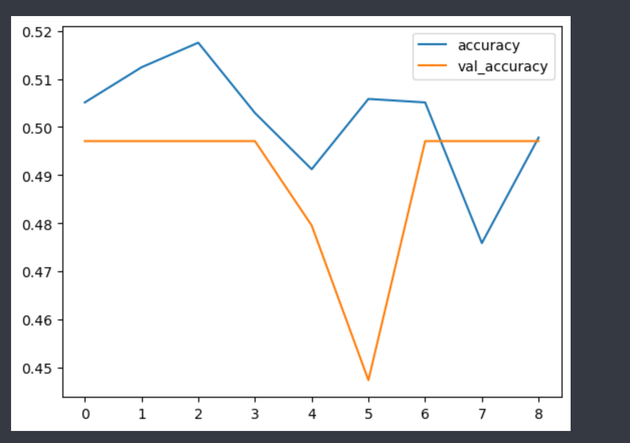
loss accuracy val_loss val_accuracy
0 0.941182 0.505117 0.945245 0.497076
1 0.942451 0.512427 0.946420 0.497076
2 0.944342 0.517544 0.949780 0.497076
3 0.944913 0.502924 0.945130 0.497076
4 0.949079 0.491228 0.995339 0.479532
5 0.950846 0.505848 0.948766 0.447368
6 0.944535 0.505117 0.967566 0.497076
7 0.949653 0.475877 0.960229 0.497076
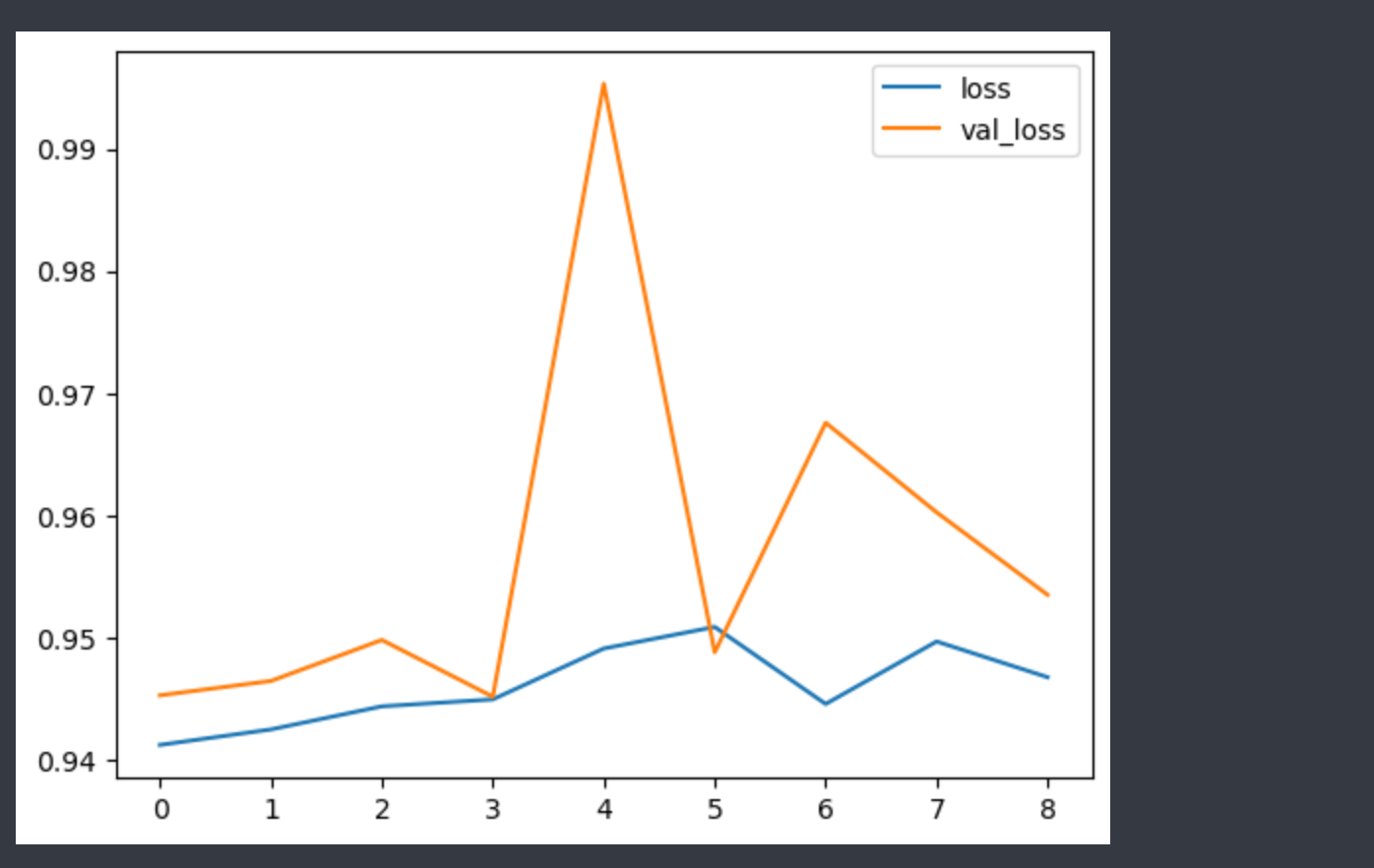
8 0.946728 0.497807 0.953476 0.497076- 시각화
예측
y_pred = model.predict(X_test_sp)평가
# np.argmax를 이용해 가장 큰 값의 인덱스들을 반환한 값(클래스 예측)을 y_predict에 할당
y_predict = np.argmax(y_pred, axis=1)

# np.argmax를 이용해 가장 큰 값의 인덱스들을 반환한 값을 y_test_val에 할당
y_test_val = np.argmax(y_test.values, axis=1)

# 맞춘 값의 평균
(y_test_val == y_predict).mean()
>>>>
0.514018691588785

loss, accuracy = model.evaluate(X_test_sp, y_test)
loss, accuracy
>>>>
(0.945652961730957, 0.514018714427948)
📍 Bidirectional LSTM
- Bidirectional 순환 신경망은 길이가 정해진 데이터 순열을 통해 어떤 값이 들어오기 전과 후의 정보를 모두 학습하는 방식의 알고리즘
- 이를 위해 순열을 왼쪽에서 오른쪽으로 읽을 RNN 하나와, 오른쪽에서 왼쪽으로 읽을 RNN 하나를 필요로 한다.
model = Sequential()
# 입력-임베딩 층
model.add(Embedding(input_dim=vocab_size,
                    output_dim=embedding_dim,
                    input_length=max_length))
model.add(Bidirectional(LSTM(units=64, return_sequences=True)))
model.add(Bidirectional(LSTM(units=64, return_sequences=True)))
model.add(Bidirectional(LSTM(units=64)))
model.add(Dense(units=16))
# 출력층
model.add(Dense(units=n_class, activation='softmax'))
model.summary()
>>>>
Model: "sequential_22"
_________________________________________________________________
 Layer (type)                Output Shape              Param #
=================================================================
 embedding_5 (Embedding)     (None, 500, 64)           64000

 bidirectional_19 (Bidirecti  (None, 500, 128)         66048
 onal)

 bidirectional_20 (Bidirecti  (None, 500, 128)         98816
 onal)

 bidirectional_21 (Bidirecti  (None, 128)              98816
 onal)

 dense_33 (Dense)            (None, 16)                2064

 dense_34 (Dense)            (None, 3)                 51

=================================================================
Total params: 329,795
Trainable params: 329,795
Non-trainable params: 0
_________________________________________________________________
compile
model.compile(optimizer='adam',
            loss='categorical_crossentropy',
            metrics=['accuracy'])
학습
history = model.fit(X_train_val, y_train_val, validation_data=(X_valid, y_valid),
			epochs=100, callbacks=[early_stop])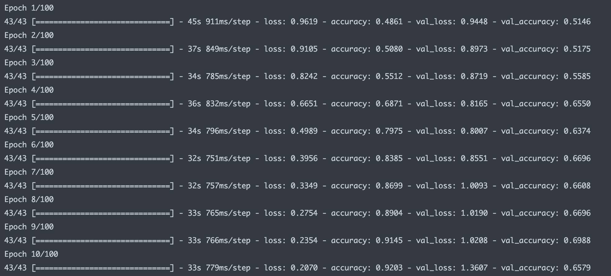
📍 GRU
- LSTM을 변형시킨 알고리즘으로 Gradient Vanishing 문제를 해결
model = Sequential()

# 입력-임베딩 층
model.add(Embedding(input_dim=vocab_size,
                    output_dim=embedding_dim,
                    input_length=max_length))
model.add(Bidirectional(GRU(units=64, return_sequences=True)))
model.add(Bidirectional(GRU(units=64)))
model.add(Dense(units=16))
# 출력층
model.add(Dense(units=n_class, activation='softmax'))
model.summary()

>>>>
Model: "sequential_24"
_________________________________________________________________
 Layer (type)                Output Shape              Param #
=================================================================
 embedding_7 (Embedding)     (None, 500, 64)           64000

 bidirectional_24 (Bidirecti  (None, 500, 128)         49920
 onal)

 bidirectional_25 (Bidirecti  (None, 128)              74496
 onal)

 dense_37 (Dense)            (None, 16)                2064

 dense_38 (Dense)            (None, 3)                 51

=================================================================
Total params: 190,531
Trainable params: 190,531
Non-trainable params: 0
_________________________________________________________________
compile
model.compile(optimizer='adam',
            loss='categorical_crossentropy',
            metrics=['accuracy'])
학습
history = model.fit(X_train_val, y_train_val, validation_data=(X_valid, y_valid),
			epochs=100, callbacks=[early_stop])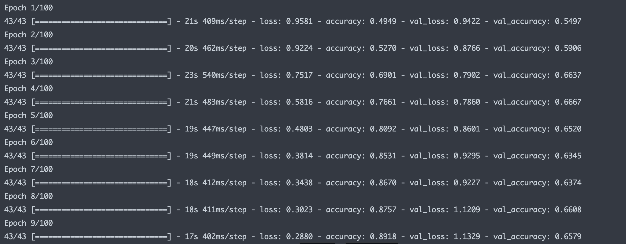
df_hist = pd.DataFrame(history.history)
df_hist
>>>>

	loss		accuracy	val_loss	val_accuracy
0	0.958088	0.494883	0.942238	0.549708
1	0.922429	0.527047	0.876623	0.590643
2	0.751728	0.690058	0.790169	0.663743
3	0.581616	0.766082	0.786014	0.666667
4	0.480338	0.809211	0.860106	0.652047
5	0.381432	0.853070	0.929460	0.634503
6	0.343799	0.866959	0.922687	0.637427
7	0.302327	0.875731	1.120898	0.660819
8 0.288006 0.891813 1.132852 0.657895- 시각화
fig, axes = plt.subplots(ncols=2, figsize=(10, 5))
df_hist[['loss', 'val_loss']].plot(ax=axes[0])
df_hist[['accuracy', 'val_accuracy']].plot(ax=axes[1])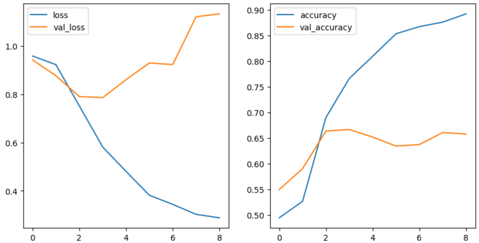
예측
y_pred = model.predict(X_test_sp)평가
y_predict = np.argmax(y_pred, axis=1)
y_test_val = np.argmax(y_test.values, axis=1)

(y_test_val == y_predict).mean()
>>>>
0.6658878504672897
✅ SimpleRNN - accuracy : 0.514018691588785
✅ GRU - accuracy : 0.6658878504672897
➡️ 확실히 성능이 좋아졌다.
정리
📌 텍스트 데이터 벡터화 하는 방법 ??
- 토큰화(str.split()) => one-hot-encoding
- bag of words (min_df, max_df, analyzer, stopwords, n-gram) - RNN은 순서가 있는 데이터를 예측할 때 주로 사용하는 데 BOW 순서를 보존하지 않는다. 그래서 시퀀스 방식의 인코딩을 사용
- Embedding => 여러 각도에서 단어와 단어 사이의 거리를 본다. 가까운 거리에 있는 단어는 유사한 단어이고 거리가 멀수록 의미가 먼 단어
-> 의미를 좀 더 보존할 수 있게 된다.
📌 텍스트 데이터 전처리 방법??
- 정규표현식 -> 텍스트 정규화
- 불용어 -> 나, 너, 그것, 이것, 저것 처럼 자주 등장하지만 큰 의미를 갖지 않는 단어 제외
- 형태소 분석 : 의미가 없는 조사, 어미, 구두점 등을 제거
- 어간 추출 (Stemming) : 원형 보존하지 않음
- 표제어 표기법 (Lemmatization) : 원형 보존함
📌 RNN
- time-step을 갖는 데이터에 주로 사용 (예시 : 자연어(챗봇), 음성, 시계열 데이터(주가 데이터), 심전도 데이터)
- RNN, LSTM, GRU
- BPTT