모델을 정의 하는 방법!

1. Sequencial 사용하기
2. Functional API model
3. Sub class model

Convolutional Neural Network

Convolutional Neural Network

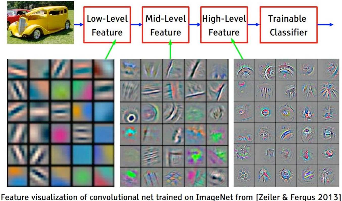
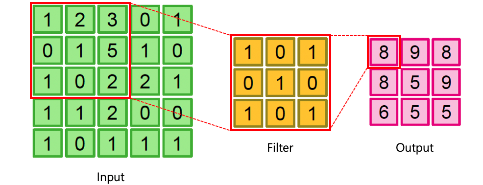
Filter to an image (Convolution layer)

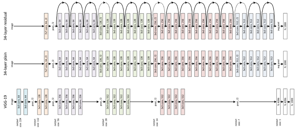
VGGNet

VGGNet은 2014년 ILSVRC에서 비록 다음에 배울 GoogLeNet에 밀려 2위를 했지만, 훨씬 간단한 구조로 이해와 변형이 쉽다는 장점이 있어 많이 응용된 모델이다.
VGGNet의 개발자들은 모델의 깊이가 성능에 얼마나 영향을 끼칠지에 집중하여 연구하였다고 논문에서 밝혔다. 깊은 네트워크를 가지고 있지만, GoogLeNet과 비교하면, 구조가 매우 간단하다. 깊이에 따른 변화를 비교하기 위해, 3x3의 작은 필터 크기를 사용했고, 모델 깊이와 구조에 변화를 주어 실험하였다. 논문에서 언급한 것은 총 6개의 모델로 내용은 다음 표와 같다. 표의 "D" 구조를 VGG16, "E" 구조를 VGG19라고 부른다. 다음 표에서, "conv 3, 64" 는 3x3 컨볼루션(convolution) 연산에 출력 피쳐맵 갯수는 64개라는 뜻이다.

A	A-LRN	B	C	D	E
11개의 레이어	11개의 레이어	13개의 레이어	16개의 레이어	16개의 레이어	19개의 레이어
conv 3, 64	conv 3, 64	conv 3, 64	conv 3, 64	conv 3, 64	conv 3, 64
	LRN	conv 3, 64	conv 3, 64	conv 3, 64	conv 3, 64
maxpool 2	maxpool 2	maxpool 2	maxpool 2	maxpool 2	maxpool 2
conv 3, 128	conv 3, 128	conv 3, 128	conv 3, 128	conv 3, 128	conv 3, 128
		conv 3, 128	conv 3, 128	conv 3, 128	conv 3, 128
maxpool 2	maxpool 2	maxpool 2	maxpool 2	maxpool 2	maxpool 2
conv 3, 256	conv 3, 256	conv 3, 256	conv 3, 256	conv 3, 256	conv 3, 256
conv 3, 256	conv 3, 256	conv 3, 256	conv 3, 256	conv 3, 256	conv 3, 256
			conv 1, 256	conv 3, 256	conv 3, 256
					conv 3, 256
maxpool 2	maxpool 2	maxpool 2	maxpool 2	maxpool 2	maxpool 2
conv 3, 512	conv 3, 512	conv 3, 512	conv 3, 512	conv 3, 512	conv 3, 512
conv 3, 512	conv 3, 512	conv 3, 512	conv 3, 512	conv 3, 512	conv 3, 512
			conv 1, 512	conv 3, 512	conv 3, 512
					conv 3, 512
maxpool 2	maxpool 2	maxpool 2	maxpool 2	maxpool 2	maxpool 2
conv 3, 512	conv 3, 512	conv 3, 512	conv 3, 512	conv 3, 512	conv 3, 512
conv 3, 512	conv 3, 512	conv 3, 512	conv 3, 512	conv 3, 512	conv 3, 512
			conv 1, 512	conv 3, 512	conv 3, 512
					conv 3, 512
maxpool 2	maxpool 2	maxpool 2	maxpool 2	maxpool 2	maxpool 2
FCN 4096	FCN 4096	FCN 4096	FCN 4096	FCN 4096	FCN 4096
FCN 4096	FCN 4096	FCN 4096	FCN 4096	FCN 4096	FCN 4096
FCN 1000	FCN 1000	FCN 1000	FCN 1000	FCN 1000	FCN 1000

Dataloader

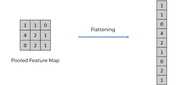
• Flatten → 채널 차원 추가로 변경

Convolution Layer는 주로 이미지 데이터 처리를 위해 사용되기 때문에, 컬러이미지는 (height, width, 3) 흑백은 (height, width, 1)로 사용한다.

ex) (num_data, 28, 28) → (num_data, 28, 28, 1)

import numpy as np
import pandas as pd
import tensorflow as tf

import matplotlib.pyplot as plt
import seaborn as sns
%matplotlib inline

np.random.seed(7777)
tf.random.set_seed(7777)

class DataLoader():

    def __init__(self):
        (self.train_x, self.train_y), (self.test_x, self.test_y) = tf.keras.datasets.mnist.load_data()

    def scale(self, x):
        return (x / 255.0).astype(np.float32)

    def preprocess_dataset(self, dataset):
        (feature, target) = dataset

        # scaling 
        scaled_x = np.array([self.scale(x) for x in feature])

        # Add channel axis 
        expanded_x = scaled_x[:, :, :, np.newaxis]

        # label encoding 
        ohe_y = tf.keras.utils.to_categorical(target, num_classes=10)
        
        return expanded_x, ohe_y

    def get_train_dataset(self):
        return self.preprocess_dataset((self.train_x, self.train_y))

    def get_test_dataset(self):
        return self.preprocess_dataset((self.test_x, self.test_y))

mnist_loader = DataLoader()

train_x, train_y = mnist_loader.get_train_dataset()
print(train_x.shape, train_x.dtype)
print(train_y.shape, train_y.dtype)

test_x, test_y = mnist_loader.get_test_dataset()
print(test_x.shape, test_x.dtype)
print(test_y.shape, test_y.dtype)

'''  (60000, 28, 28, 1) float32
     (60000, 10) float32
     (10000, 28, 28, 1) float32
     (10000, 10) float32

VGGNet에서 사용되는 Layer들

• tf.keras.layers.Conv2D
• tf.keras.layers.Activation
• tf.keras.layers.MaxPool2D
• tf.keras.layers.Flatten
• tf.keras.layers.Dense

Conv2D

tf.keras.layers.Conv2D()

• filters: layer에서 사용할 Filter(weights)의 갯수
• kernel_size: Filter(weights)의 사이즈
• strides: 몇 개의 pixel을 skip 하면서 훑어지나갈 것인지 (출력 피쳐맵의 사이즈에 영향을 줌)
• padding: zero padding을 만들 것인지. VALID는 Padding이 없고, SAME은 Padding이 있음 (출력 피쳐맵의 사이즈에 영향을 줌)
• activation: Activation Function을 지정

MaxPool2D

tf.keras.layers.MaxPool2D()

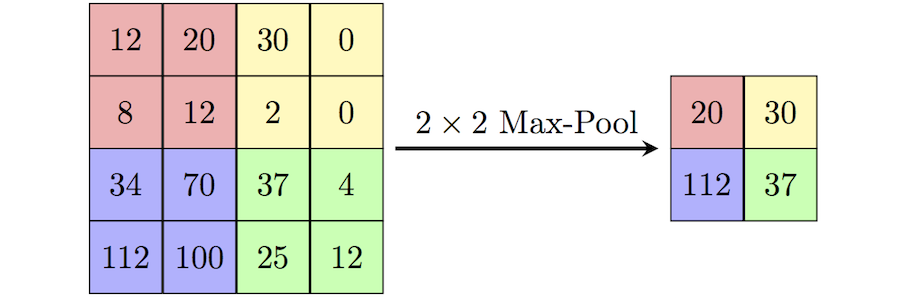
• pool_size: Pooling window 크기
• strides: 몇 개의 pixel을 skip 하면서 훑어지나갈 것인지
• padding: zero padding을 만들 것인지

Flatten

tf.keras.layers.Flatten()

Dense

tf.keras.layers.Dense()

• units : 노드 갯수
• activation : 활성화 함수
• use_bias : bias 를 사용 할 것인지
• kernel_initializer : 최초 가중치를 어떻게 세팅 할 것인지
• bias_initializer : 최초 bias를 어떻게 세팅 할 것인지

1. Sequencial 방식

from tensorflow.keras.layers import Conv2D, MaxPool2D, Flatten, Dense

model = tf.keras.Sequential()

model.add(Conv2D(32, kernel_size=3, padding='same', activation='relu', input_shape=(28, 28, 1))) 
model.add(Conv2D(32, kernel_size=3, padding='same', activation='relu'))
model.add(MaxPool2D())

model.add(Conv2D(64, kernel_size=3, padding='same', activation='relu')) 
model.add(Conv2D(64, kernel_size=3, padding='same', activation='relu'))
model.add(MaxPool2D())

model.add(Flatten())
model.add(Dense(128, activation="relu"))
model.add(Dense(64, activation="relu"))
model.add(Dense(10, activation="softmax"))

model.summary()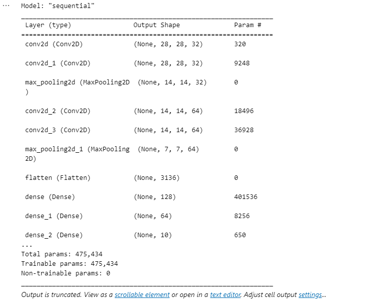

learning_rate = 0.0001
opt = tf.keras.optimizers.Adam(learning_rate)
loss = tf.keras.losses.categorical_crossentropy

model.compile(optimizer=opt, loss=loss, metrics=["accuracy"])

hist = model.fit(train_x, train_y, epochs=50, batch_size=128, validation_data=(test_x, test_y))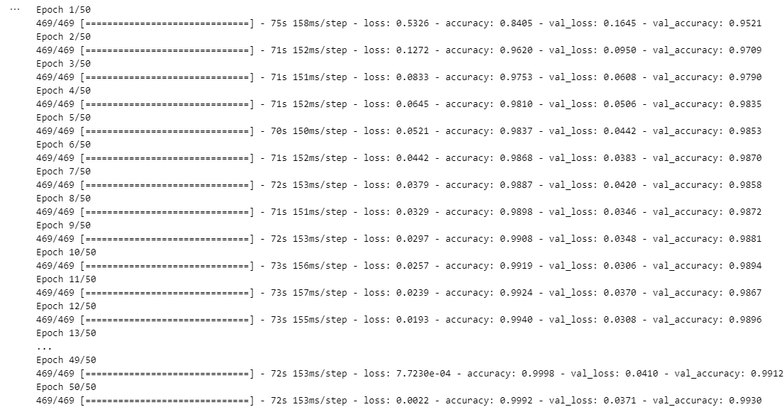

plt.figure(figsize=(10, 5))

plt.subplot(221)
plt.plot(hist.history['loss'])
plt.title("loss")

plt.subplot(222)
plt.plot(hist.history['accuracy'], 'b-')
plt.title("accuracy")

plt.subplot(223)
plt.plot(hist.history['val_loss'])
plt.title("val_loss")
plt.subplot(224)

plt.plot(hist.history['val_accuracy'], 'b-')
plt.title("val_accuracy")

plt.tight_layout()
plt.show()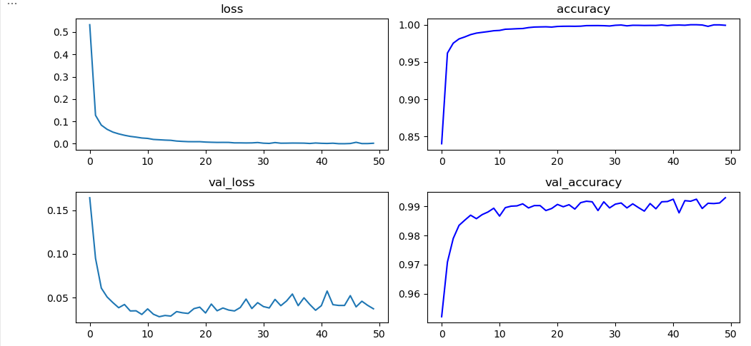

2. Functional API model

tf.keras.Sequential 보다 더 유연하게 모델을 정의할 수 있는 방법

import numpy as np
import pandas as pd
import tensorflow as tf
from tensorflow.keras.layers import Input, Conv2D, MaxPool2D, Flatten, Dense

import matplotlib.pyplot as plt
import seaborn as sns
%matplotlib inline

input_shape=(28, 28, 1)
inputs = Input(input_shape)

net = Conv2D(32, kernel_size=3, padding='same', activation='relu')(inputs)
net = Conv2D(32, kernel_size=3, padding='same', activation='relu')(net)
net = MaxPool2D()(net)

net = Conv2D(64, kernel_size=3, padding='same', activation='relu')(net)
net = Conv2D(64, kernel_size=3, padding='same', activation='relu')(net)
net = MaxPool2D()(net)

net = Flatten()(net)
net = Dense(128, activation="relu")(net)
net = Dense(64, activation="relu")(net)
net = Dense(10, activation="softmax")(net)

model = tf.keras.Model(inputs=inputs, outputs=net, name='VGG')

model.summary()

ResNet 구현

ResNet

ResNet의 핵심은 Skip Connection

2. Functional API model

tf.keras.Sequential 보다 더 유연하게 모델을 정의할 수 있는 방법

import numpy as np
import pandas as pd
import tensorflow as tf
from tensorflow.keras.layers import Input, Conv2D, MaxPool2D, Flatten, Dense

import matplotlib.pyplot as plt
import seaborn as sns
%matplotlib inline

def build_resnet(input_shape):

    inputs = Input(input_shape)

    net = Conv2D(32, kernel_size=3, strides=2, padding='same', activation='relu')(inputs)
    net = MaxPool2D()(net)
    
    net1 = Conv2D(64, kernel_size=1, padding='same', activation='relu')(net)
    net2 = Conv2D(64, kernel_size=3, padding='same', activation='relu')(net1)
    net3 = Conv2D(64, kernel_size=1, padding='same', activation='relu')(net2)
    
    net1_1 = Conv2D(64, kernel_size=1, padding='same')(net)
    net = Add()([net1_1, net3])
    
    net1 = Conv2D(64, kernel_size=1, padding='same', activation='relu')(net)
    net2 = Conv2D(64, kernel_size=3, padding='same', activation='relu')(net1)
    net3 = Conv2D(64, kernel_size=1, padding='same', activation='relu')(net2)
    
    net = Add()([net, net3])
    
    net = MaxPool2D()(net)
    
    net = Flatten()(net)
    net = Dense(10, activation="softmax")(net)

    model = tf.keras.Model(inputs=inputs, outputs=net, name='resnet')
    
    return model

model = build_resnet((32, 32, 3))
model.summary()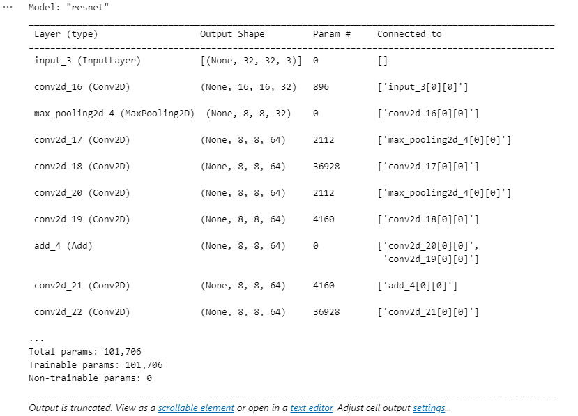

CIfar10 dataset을 이용해 학습

class Cifar10DataLoader():

    def __init__(self):
        # data load
        (self.train_x, self.train_y),(self.test_x, self.test_y) = tf.keras.datasets.cifar10.load_data()
        self.input_shape = self.train_x.shape[1:]

    def scale(self, x):
        return (x / 255.0).astype(np.float32)

    def preprocess_dataset(self, dataset):
        (feature, target) = dataset

        # scaling 
        scaled_x = np.array([self.scale(x) for x in feature])

        # label encoding 
        ohe_y = tf.keras.utils.to_categorical(target, num_classes=10)

        return scaled_x, ohe_y

    def get_train_dataset(self):
        return self.preprocess_dataset((self.train_x, self.train_y))

    def get_test_dataset(self):
        return self.preprocess_dataset((self.test_x, self.test_y))

cifar10_loader = Cifar10DataLoader()

train_x, train_y = cifar10_loader.get_train_dataset()
print(train_x.shape, train_x.dtype)
print(train_y.shape, train_y.dtype)

test_x, test_y = cifar10_loader.get_test_dataset()
print(test_x.shape, test_x.dtype)
print(test_y.shape, test_y.dtype)

'''   (50000, 32, 32, 3) float32
      (50000, 10) float32
      (10000, 32, 32, 3) float32
      (10000, 10) float32

learning_rate = 0.001
opt = tf.keras.optimizers.Adam(learning_rate)
loss = tf.keras.losses.categorical_crossentropy

model.compile(optimizer=opt, loss=loss, metrics=["accuracy"])

hist = model.fit(train_x, train_y, epochs=50, batch_size=128, validation_data=(test_x, test_y))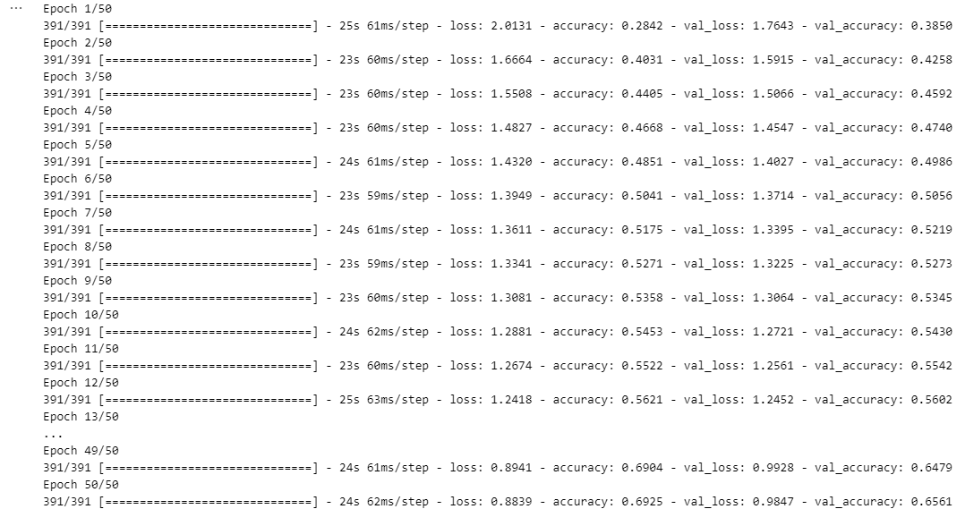

plt.figure(figsize=(12, 10))

plt.subplot(221)
plt.plot(hist.history['loss'])
plt.title("loss")

plt.subplot(222)
plt.plot(hist.history['accuracy'], 'b-')
plt.title("accuracy")

plt.subplot(223)
plt.plot(hist.history['val_loss'])
plt.title("val_loss")

plt.subplot(224)
plt.plot(hist.history['val_accuracy'], 'b-')
plt.title("val_accuracy")

plt.tight_layout()
plt.show()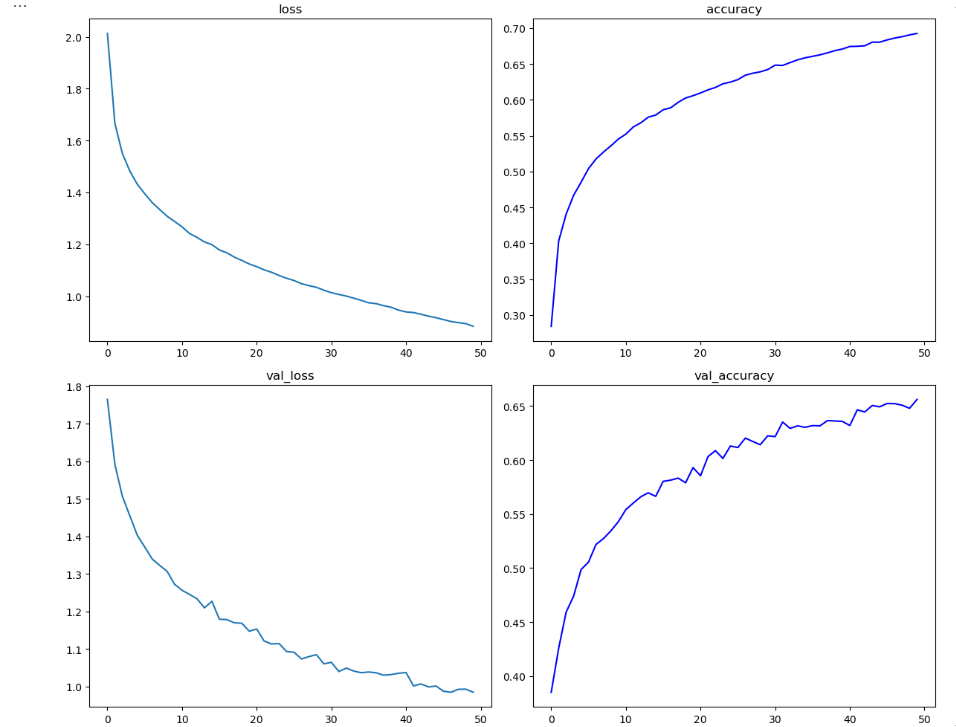

3. Sub class model

모델 이란 것은 Input을 Output으로 만들어주는 수식이다.

해당 기능을 수행하는 두 가지 클래스가 tf.keras.layers.Layer 와 tf.keras.layers.Model 클래스이다.

두가지 모두 연산을 추상화 하는 것으로 동일한 역할을 하지만, tf.keras.layers.Model 클래스의 경우 모델을 저장 하는 기능 과 fit 함수를 사용할 수 있다는 점에서 차이가 있다.

• tf.keras.layers.Layer
• tf.keras.layers.Model

Linear Regression을 Layer로 만들어 보자.

class LinearRegression(tf.keras.layers.Layer):

    def __init__(self, units):
        super(LinearRegression, self).__init__()
        self.units = units

    def build(self, input_shape):
        self.w = self.add_weight(
            shape=(input_shape[-1], self.units),
            initializer="random_normal",
            trainable=True,
        )
        self.b = tf.Variable(0.0)

    def call(self, inputs):
        return tf.matmul(inputs, self.w) + self.b

가상 데이터

W_true = np.array([[3., 2., 4., 1.]]).reshape((4, 1))
B_true = np.array([1.])

X = tf.random.normal((500, 4))
noise = tf.random.normal((500, 1))

y = X @ W_true + B_true + noise

opt = tf.keras.optimizers.SGD(learning_rate=3e-2)

linear_layer = LinearRegression(1)

for epoch in range(100):

    with tf.GradientTape() as tape:
        y_hat = linear_layer(X)
        loss = tf.reduce_mean(tf.square((y - y_hat)))
        
    grads = tape.gradient(loss, linear_layer.trainable_weights)
    
    opt.apply_gradients(zip(grads, linear_layer.trainable_weights))
    
    if epoch % 10 == 0:
        print("epoch : {} loss : {}".format(epoch, loss.numpy()))

ResNet - Sub Class 로 구현 하기

1. Residual Block - Layer
2. ResNet - Model

import numpy as np
import pandas as pd
import tensorflow as tf
from tensorflow.keras.layers import Input, Conv2D, MaxPool2D, Flatten, Dense

import matplotlib.pyplot as plt
import seaborn as sns
%matplotlib inline

class ResidualBlock(tf.keras.layers.Layer):

    def __init__(self, filters=32, filter_match=False):
        super(ResidualBlock, self).__init__()
    
        self.conv1 = Conv2D(filters, kernel_size=1, padding='same', activation='relu')
        self.conv2 = Conv2D(filters, kernel_size=3, padding='same', activation='relu')
        self.conv3 = Conv2D(filters, kernel_size=1, padding='same', activation='relu')
        self.add = Add()
        
        self.filters = filters
        self.filter_match = filter_match
        if filter_match:
            self.conv_ext = Conv2D(filters, kernel_size=1, padding='same')
        
    def call(self, inputs):
        net1 = self.conv1(inputs)
        net2 = self.conv2(net1)
        net3 = self.conv3(net2)
        if self.filter_match:
            res = self.add([self.conv_ext(inputs), net3])
        else: 
            res = self.add([inputs, net3])
        return res 

class ResNet(tf.keras.Model):

    def __init__(self, num_classes):
        super(ResNet, self).__init__()
        
        self.conv1 = Conv2D(32, kernel_size=3, strides=2, padding='same', activation='relu')
        self.maxp1 =  MaxPool2D()
        self.block_1 = ResidualBlock(64, True)
        self.block_2 = ResidualBlock(64)
        self.maxp2 =  MaxPool2D()
        self.flat = Flatten()
        self.dense = Dense(num_classes)

    def call(self, inputs):
        x = self.conv1(inputs)
        x = self.maxp1(x)
        x = self.block_1(x)
        x = self.block_2(x)
        x = self.maxp2(x)
        x = self.flat(x)
        return self.dense(x)

model = ResNet(num_classes=10)

학습 시켜보기

class Cifar10DataLoader():

    def __init__(self):
        # data load
        (self.train_x, self.train_y), (self.test_x, self.test_y) = tf.keras.datasets.cifar10.load_data()
        self.input_shape = self.train_x.shape[1:]

    def scale(self, x):
        return (x / 255.0).astype(np.float32)

    def preprocess_dataset(self, dataset):
        (feature, target) = dataset

        # scaling 
        scaled_x = np.array([self.scale(x) for x in feature])

        # label encoding 
        ohe_y = np.array([tf.keras.utils.to_categorical(
            y, num_classes=10) for y in target])
        
        return scaled_x, ohe_y.squeeze(1)

    def get_train_dataset(self):
        return self.preprocess_dataset((self.train_x, self.train_y))

    def get_test_dataset(self):
        return self.preprocess_dataset((self.test_x, self.test_y))

cifar10_loader = Cifar10DataLoader()

train_x, train_y = cifar10_loader.get_train_dataset()

print(train_x.shape, train_x.dtype)
print(train_y.shape, train_y.dtype)

test_x, test_y = cifar10_loader.get_test_dataset()

print(test_x.shape, test_x.dtype)
print(test_y.shape, test_y.dtype)

'''   (50000, 32, 32, 3) float32
      (50000, 10) float32
      (10000, 32, 32, 3) float32
      (10000, 10) float32

learning_rate = 0.001
opt = tf.keras.optimizers.Adam(learning_rate)
loss = tf.keras.losses.categorical_crossentropy

model.compile(optimizer=opt, loss=loss, metrics=["accuracy"])

hist = model.fit(train_x, train_y,
                 epochs=10, 
                 batch_size=128,
                 validation_data=(test_x, test_y))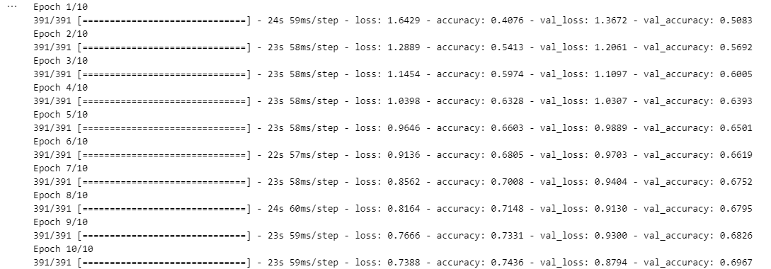

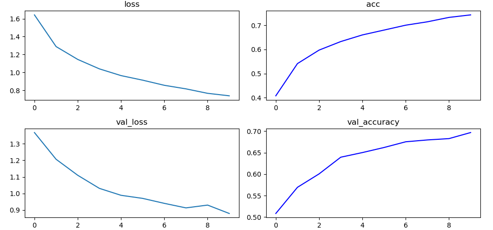
plt.figure(figsize=(10, 5))

plt.subplot(221)
plt.plot(hist.history['loss'])
plt.title("loss")

plt.subplot(222)
plt.plot(hist.history['accuracy'], 'b-')
plt.title("acc")

plt.subplot(223)
plt.plot(hist.history['val_loss'])
plt.title("val_loss")

plt.subplot(224)
plt.plot(hist.history['val_accuracy'], 'b-')
plt.title("val_accuracy")

plt.tight_layout()
plt.show()