A survey on model-based reinforcement learning

결·2025년 5월 8일

목록 보기

11/11

1. Overview of model-based RL

Therefore, applying RL algorithms with high sample complexity to real-world tasks is diﬃcult, where trial-and-error can be extremely expensive.

→ RL알고리즘을 high sample complexity에 적용하는 게 어렵다.

Therefore, a major focus of recent deep RL (DRL) research has been on enhancing sample eﬃciency [5]. Model-based RL (MBRL) is one of the most important research directions that have the potential to make
RL algorithms significantly more sample eﬃcient [6].

→ 따라서, sample을 efficient하게 하려면 model-based RL이 필요

→ 수천 번의 가상 상호작용을 빠르게 수행

MDP는 ⟨S, A, M, R, γ⟩로 이루어진다.

S : state space
A : action space
γ : discount factor for future rewards
M : S ×A →S - state transition dynamics
R : S ×A - reward function

그래서, "모델을 학습한다"의 의미는, M과 R을 recover한다는 뜻.
이미 많은 경우에 reward function은 이미 define되어있으니까,
사실상, 주요 목표는 state transition dynamics인 M을 학습하는 게 주요 목표겠지!

이렇게 하면 샘플 복잡도가 줄어들고, 모델에서 생성된 시뮬레이션 데이터를 통해 학습을 하게 되는 것.
이때, 이 시뮬레이션 데이터를 활용해서 policy를 학습하게 되는 것이다!

Recent studies from both theoretical [14] and empirical [6, 8] perspectives demonstrate that, given
a suﬃciently accurate model, it is intuitive that MBRL yields higher sample eﬃciency than MFRL.
-> 일단 accurate한 모델이 있다면, MBRLd은 sample efficiency가 더 높다 MFRL보다는...

그리고 이 Model-based RL이 2가지로 나뉠 수 있다.

blackbox model rollout for trajectory sampling
whitebox model for gradient propagation

게다가, Model-based와 다른 애들이 합쳐진 걸 또 배울 것이다.
(OffRL, multi-agent RL 등등)

2 Model Learning

We assume that some historical
data is available for learning. Usually, the historical data can be in the form of trajectories {τ1, τ2, . . . , τk },
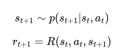
and each trajectory is a sequence of state-action-reward pairs

M : (st, at) -> (st+1)
R : (st, at) -> rt

2.1 Model Learning in tabular setting

단순히 Tabular setting이라고 한다면,

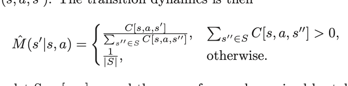
(s,a)를 집어넣었을때,
ex) (s,a,s1):3번 (s,a,s2): 4번 (s,a,s3):5번
(s,a)를 넣었을때, s1이 나올 확률은?
= 3/(3+4+5)가 되는 거지,

Notice that

\hat{M}, \hat{R}

are an unbiased
estimation of the true transition

M^* R^*

respectively, and thus converge to
them as the samples approach infinity.
-> 결국 추정치지만 나중에는 infinity로 수렴

A key limitation of the
analysis is the assumption of the tabular setting, where models are not able to generalize across states.
-> 근데, 이 Tabular setting의 중요한 점은,
상태들 간의 일반화를 하지 못한다
: 상태가 매우 적고 고정되어 있는 경우에는 잘 작동 but 상태 공간이 커지거나 복잡해지면 효율적X
=> 상태 간의 연결 관계나 패턴을 파악하지 못한다

예를 들어서, 상태 간 일반화가 이루어지지 않기 때문에 상태 A와 상태 C가 유사하다고 해도, 이를 따로 다룰 수밖에 없음.

P(s ′ ∣A,a)≈P(s ′ ∣C,a) for some s ′ ∈S

Q(A,a)=R(A,a)+γ \underset{a ′}max​Q(s ′ ,a ′ )

Q ( C , a ) = R ( C , a ) + γ \underset{a ′} max Q ( s ′ , a ′ )

이런식으로 일반화가 될 수 있다.!
근데 Tabular setting에서는,
독립적으로 값이 계산이 되는거지.

2.2 Model Learning via prediction loss

linear model들로 이제 approximation을 한다.

M_θ(approximation) 와 M^∗(real)

2.2.1 Prediction model loss

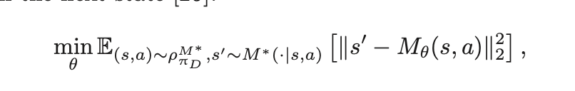
1) the stationary
state-action distribution induced by πD and M ∗
로부터 뽑은 (s,a)를 approximation에 넣은 다음에 나오는 state
2) M*(.|(s,a))로부터 뽑은 s'
을 가지고
MSE를 구하는 거다.

근데 이렇게 되면 어떤 문제가 생긴다?

=> 바로 특정 하나의 s'로 전이가 된다.

M(s'|(s,a))

얘가 무조건 s'으로 되는가? ㄴㄴ
그럼 이것도 확률분포가 되는거.

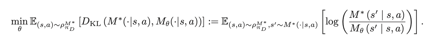
그래서 단순히, s'으로 나오는 게 아니니까 MSE를 쓰지 말고 KL divergence를 활용해보자고요~! (분포와 분포사이의 척도를 재는 KL divergence)

근데, 이때, M_θ가 보통 가우시안으로 정의가 되기 때문에

결국에는, 저 식으로 된다.
그래서 어떤 supervised learning이라도 사용될 수 있는 이유임.

2.2.2 Model Properties

수학적으로는, 시간이 지날수록 오차가 2차적으로 더 커진다. 그러니 실제환경이랑 매우 일치해야한다.

2.2.3 Model Variants

<단계별 모델>

기존의 전통적인 모델
: 한 번에 하나의 상태를 예측
: 이 모델은 예측한 상태를 다시 입력으로 사용하는 구조 => 누적 오차(compounding error) 발생 가능
단계별 모델(multistep model)
: 한 번에 여러 단계를 예측
: "가짜" 상태를 입력으로 사용하지 않으니까 => 오차가 누적되지 않음.

<역방향 전이 모델>

기존 모델
s_t와 a_t를 입력으로 받아서 s_t+1예측하기
역방향 전이 모델
s_t+1과 a_t를 입력으로 받아서 s_t예측하기

2.3 Model Learning with reduced error

2.3.1 Model learning with Lipschitz continuity constraint

: 일단 아까 compounding error(계속해서 누적되는 error)가 생기니까, 그걸 없애줘야겠지?
활용한 것 1 : Lipschitz continuity constraint

활용한 것 2 : Wasserstein 거리
== 두 확률분포 P와 Q 사이의 "최소한의 이동 비용" 개념

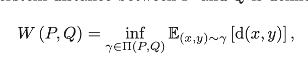
(이때, Π (P, Q) denotes the set of all joint distributions γ(x, y))
( γ에서 x만 봤을 때 나오는 분포가 P, γ에서 y만 봤을 때 나오는 분포가 Q

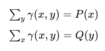
이렇게 생각하면 될듯.

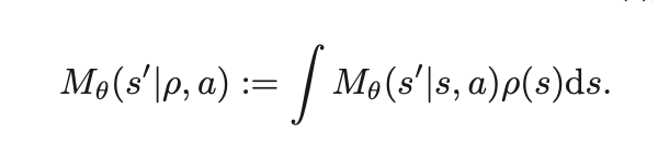
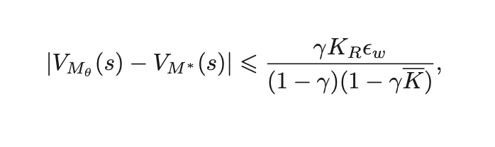
그래서, a state distribution ρ over the state space S 를 고려해봤을 때, state transition dynamics를 이렇게 정의할 수 있다 :

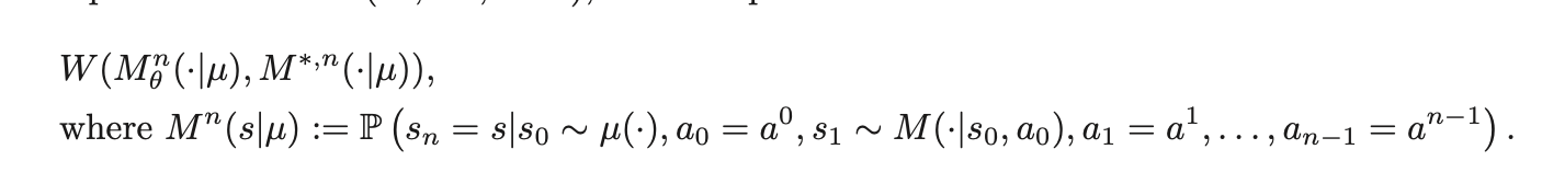
근데, 중요한 건 그러면 n-step error가 있을 때 upperbound가 뭐니 뭥미 이거잖아?

2.3.2 Model learning by distribution matching

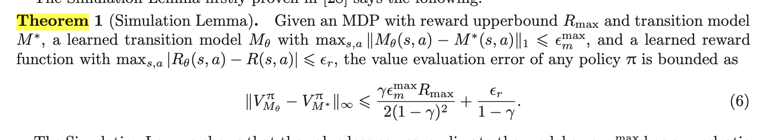
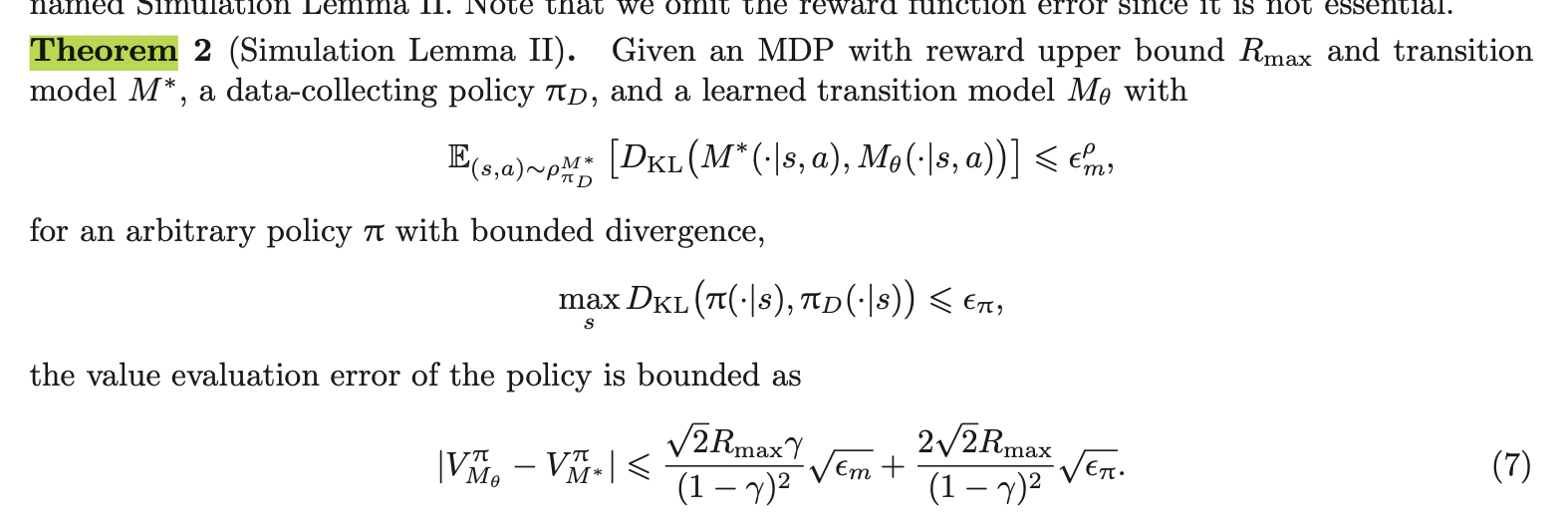
The prediction loss employed in Theorems 1 and 2 minimizes the model error on each point of the
state-action data. While the prediction loss minimization can be straightforwardly solved by supervised
learning, the long-term eﬀect of transitions is hard to capture, resulting in the horizon-squared com-
pounding error issue.
=> "이 한 번의 예측"만 잘하면 되는 게 아님!
=> n-step 시뮬레이션이 중요
=> 그러니, match the distributions between the real trajectories and the trajectories rolled out in the learned model. ! ! ! ! !
=> 매칭을 시키자.

Model-based로 만들어낸 데이터랑 기존 데이터상의 분포 mismatch가 일어날 거 아니니!
그래서, phi(E) 즉, expert data로부터 온 (s,a)를 활용해서 log(D(s,a)) + phi(phi) 즉, 에이전트 만든 data로부터 온 (s,a)를 활용해서 만든 log(1-D(s,a))를 maximize해야한다.

결

한발한발 나아갑니당!

이전 포스트