
Logistic Regression
- Why?
- 분류 문제는 0 또는 1로 예측 해야하지만 Linear Regression 적용하면 예측값이 0보다 작거나 1보다 큰 값을 가질 수 있음
- 가 항상 0에서 1 사이의 값을 갖도록 함수를 수정
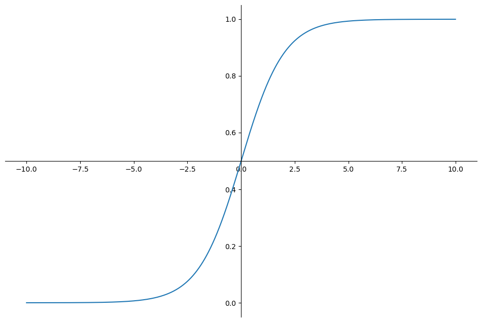
- 0과 1로 수렴!
- 해석
- 로지스틱회귀에서 는 에서 1이 될 확률을 의미
- 그니깐 종양이 악성일 확률을 말한다!
- Classification Hypothesis
- 1(악성) 으로 예측
- 0(양성) 으로 예측
- Cost Function
- 다양한 형태의 분류식이 있다
- 하지만 cost function을 계산하기에 쉽지 않다
- Logistic Regression 은 0과 1 기준으로 Cost Function을 정의 할 수 있다.
-
Learning Rate 는 기존과 동일!
-
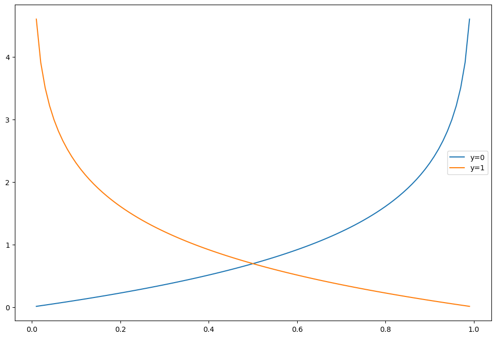
Logistic Regrssion Cost Function Graph
-
, 이 다른 형태인 것을 볼 수 있다
- Decsion Tree와 비교
- Python
import pandas as pd

url = 'https://raw.githubusercontent.com/PinkWink/ML_tutorial/master/dataset/wine.csv'

wine = pd.read_csv(url, index_col=0)
wine['taste'] = [1 if grade > 5 else 0 for grade in wine['quality']]

X = wine.drop(['taste','quality'], axis = 1)
y = wine['taste']

from sklearn.model_selection import train_test_split

X_train, X_test, y_train, y_test = train_test_split(X, y,
                                                    test_size=0.2,
                                                    random_state=13)

from sklearn.linear_model import LogisticRegression
from sklearn.metrics import accuracy_score
from sklearn.pipeline import Pipeline
from sklearn.preprocessing import StandardScaler
from sklearn.tree import DecisionTreeClassifier

models = {'logistic regression' : pipe , 'decision tree':wine_tree}- 예측 및 그래프 그리기
from sklearn.metrics import roc_curve

plt.figure(figsize=(10,8))
plt.plot([0,1],[0,1])
for mode1_name, mode1 in models.items():
    pred = mode1.predict_proba(X_test)[:,1]
    fpr, tpr, thresholds = roc_curve(y_test, pred)
    plt.plot(fpr, tpr, label=mode1_name)

plt.grid()
plt.legend()
plt.show()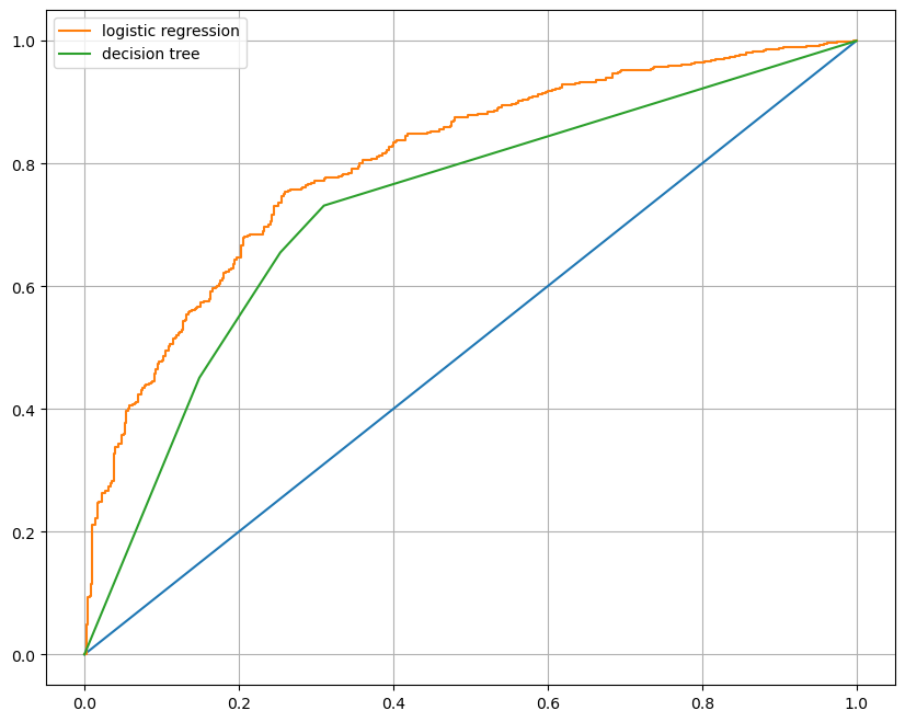
- Logistic regression의 AUC 커브의 넓이가 넓어진 것을 볼 수 있다
PIMA 데이터 당뇨병 예측
- 몇가지 잡기술만 기억해둘 필요가 있기 때문에 빠르게 skip!
- 데이터 읽기
import pandas as pd

url = 'https://raw.githubusercontent.com/PinkWink/ML_tutorial/master/dataset/diabetes.csv'

pima = pd.read_csv(url)- (EDA) 상관관계 확인
import seaborn as sns
import matplotlib.pyplot as plt

plt.figure(figsize=(12,10))
sns.heatmap(df.corr(), annot=True,cmap ='YlGnBu');- (EDA) 컬럼 타입 변경 및 0값 평균으로 변경
(df==0).astype(int).sum()

zero_features = ['Glucose', 'BloodPressure', 'SkinThickness', 'BMI']
df[zero_features] = df[zero_features].replace(0, df[zero_features].mean())

(df==0).astype(int).sum()- 분석시작
from sklearn.model_selection import train_test_split

X = df.drop(['Outcome'], axis = 1)
y = df['Outcome']

X_train, X_test ,y_train, y_test = train_test_split(X, y,
                                                     test_size= 0.2,
                                                     stratify= y,
                                                     random_state= 13)
                                         from sklearn.pipeline import Pipeline
from sklearn.preprocessing import StandardScaler
from sklearn.linear_model import LogisticRegression

estimator = [('sckaer' , StandardScaler()),
              ('clf', LogisticRegression(solver='liblinear', random_state=13))]

pipe_lr = Pipeline(estimator)
pipe_lr.fit(X_train, y_train)
pred = pipe_lr.predict(X_test) - 결과 확인
from sklearn.metrics import accuracy_score, recall_score, precision_score, roc_auc_score, f1_score

print(f'Accuracy : {accuracy_score(y_test, pred)}')
print(f'Recall : {recall_score(y_test, pred)}')
print(f'Precision : {precision_score(y_test, pred)}')
print(f'AUC score : {roc_auc_score(y_test, pred)}')
print(f'f1 Score : {f1_score(y_test, pred)}')

>>>
Accuracy : 0.7727272727272727
Recall : 0.6111111111111112
Precision : 0.7021276595744681
AUC score : 0.7355555555555556
f1 Score : 0.6534653465346535- 계수확인
coef = list(pipe_lr['clf'].coef_[0])
label = list(X_train.columns)

features  = pd.DataFrame({'feature': label , 'importance':coef})
features.sort_values(by=['importance'], ascending=True, inplace=True)-
Tree 기반은 feature importance
-
regression 기반은 coefficient?
-
그래프 그리기
features['positive'] = features['importance'] > 0
features.set_index('feature', inplace=True)

features['importance'].plot(kind='barh',
                            figsize=(11,6),
                            color = features['positive'].map({True:'blue',
                                                              False:'red'}))
plt.xlabel('Importance')
plt.show()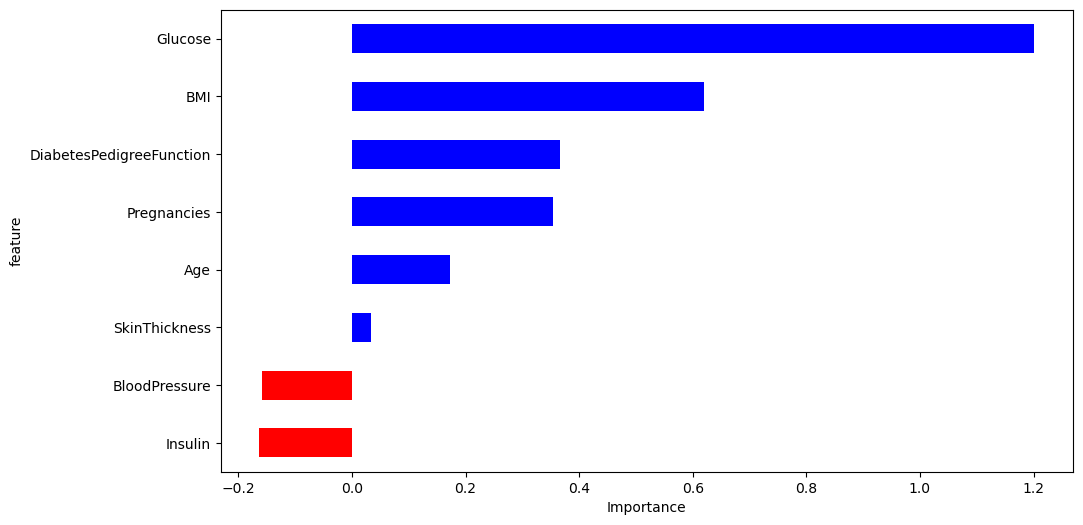

Easy day!