Graph Neural Network (2주차) (3)

박성철 | 수리데이터사이언스학과 | 한양대(ERICA) ·2026년 4월 8일

GNN 스터디

4부 : GAT

GAT는 GCN의 개선 모델
기존 GCN은 고정된 Normalization 값을 사용
GAT는 대신 self-attention으로 가중치 계산 -> 이게 핵심 차이
GCN : 이웃 다 비슷하게 봄
GAT : 중요한 이웃 더 크게 봄

GCN의 한계

GCN에서는 이웃 노드의 중요도를 degree 기반으로만 계산한다.

$\frac{1}{\sqrt{deg(i)}\sqrt{deg(j)}}$

노드의 Feature 정보는 고려하지 않음
단순히 연결 수(Degree)만으로 중요도 결정

GAT의 핵심 아이디어

이웃 노드의 중요도를 직접 학습하자

그래서 등장한 것이 attention score :

$\alpha_{ij}$

노드 i와 j사이의 중요도

Graph Attention 연산

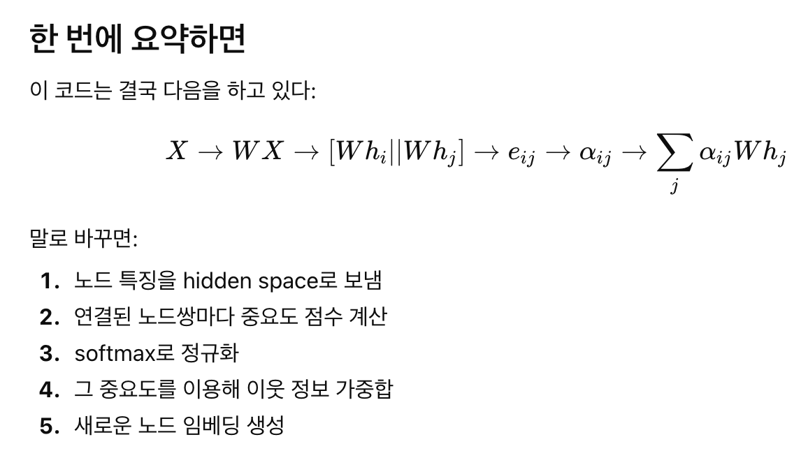
GAT의 핵심 수식:

$h_i = \sum_{j \in \mathcal{N}_i} \alpha_{ij} W x_j$

h : 노드 i의 새로운 표현
N : 노드 i의 이웃 집합
Wx : 이웃 노드 feature 변환
a : attention(중요도)

해석 :

이웃 노드 정보를 가져오되 중요도 만큼 가중합

Self-Attention의 의미

GAT에서 attention은:

노드들끼리 서로 비교해서 계산됨

Attention 계산 과정

GAT에서 attention은 다음 단계로 계산된다.
1. Linear Transformation
2. Activation Function
3. Softmax Normalization
4. Multi-head Attention
5. Improved GAT

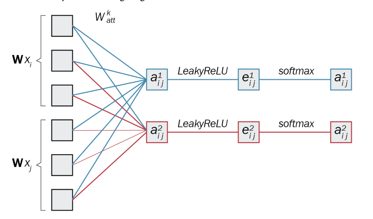
1. Linear Transformation

attention을 계산하려면 두 노드 i, j의 정보를 같이 봐야 한다.
그래서 :

$[W x_i \parallel W x_j]$

두 벡터를 concat

그리고 추가 weight 적용:

$W_{\text{att}}$

이 과정을 통해 attention score 생성:

$\alpha_{ij}$

결과 :

$a_{ij} = W_{att}^T [W x_i \parallel W x_j]$

두 노드 i, j 정보를 합쳐서 attention score의 "원재료"를 만든 것

2. Activation Function (LeakyReLU)

단순 선형 연산만 하면 -> 표현력이 부족함
그래서 비선형성(nonlinearity) 추가 필요
사용함수 : Leaky ReLU
기존 ReLU 문제 :
음수 입력 : 전부 0
뉴런이 죽는 문제

-> 해결 : LeakyReLU

음수도 조금은 살려둠

$e_{ij} = \text{LeakyReLU}(a_{ij})$

3. Softmax Normalization

문제 : Activation Function 이후에 e_ij 값들이 정규화가 안되어 서로 비교가 불가능하다. 그래서 Softmax로 확률처럼 변환해야 한다.

최종 attention score

$\alpha_{ij} = \text{softmax}_j(e_{ij}) = \frac{\exp(e_{ij})}{\sum_{k \in \mathcal{N}_i} \exp(e_{ik})}$

4. Multi-head Attention

기존 attention 문제:

attention은 불안정함 (unstable)
하나의 attention만 쓰면 결과가 편향될 수 있음

여러 개의 attention을 동시에 사용하자

핵심 아이디어 :

attention을 한 번이 아니라 여러 번 계산
각 head마다:

다른 weight
다른 attention score
각 head의 출력

각 head k는 다음과 같은 embedding 생성:

$h_i^k = \sum_{j \in \mathcal{N}_i} \alpha_{ij}^k W^k x_j$

k : attention head index

각각 독립적으로 계산됨

결과 합치는 방법

Averaging(평균)

$h_i = \frac{1}{n} \sum_{k=1}^{n} h_i^k = \frac{1}{n} \sum_{k=1}^{n} \sum_{j \in \mathcal{N}_i} \alpha_{ij}^k W^k x_j$
Concatenation (붙이기)

$h_i = \big\Vert_{k=1}^{n} h_i^k = \big\Vert_{k=1}^{n} \sum_{j \in \mathcal{N}_i} \alpha_{ij}^k W^k x_j$
규칙:

Hidden Layer : Concatenation
마지막 Layer : Averaging

Improved Graph Attention Layer (GATv2)

기존 GAT의 문제

Static Attention으로, attention이 입력에 따라 충분히 유연하게 변하지 않았다. 그래서 표현력이 제한되었다.

기존 GAT 수식 구조

$\alpha_{ij} = \frac{\exp(W_{att}^t LeakyReLU(W[x_i \parallel x_j]))}{\sum_{k \in \mathcal{N}_i} \exp(W_{att}^t LeakyReLU(W[x_i \parallel x_k]))}$

$1. [x_i || x_j] (concat)$
$2. W 적용$
$3. LeakyReLU$
$4. W_att 적용$

W가 먼저 적용된다.

GATv2 수식 구조

$\alpha_{ij} = \frac{\exp\left( \mathbf{W}_{att}^t \text{LeakyReLU}\left( \mathbf{W} [x_i \parallel x_j] \right) \right)}{\sum_{k \in \mathcal{N}_i} \exp\left( \mathbf{W}_{att}^t \text{LeakyReLU}\left( \mathbf{W} [x_i \parallel x_k] \right) \right)}$

W 적용 위치를 뒤로 이동
attention 계산 순서를 바꿈

결과
attention이 입력에 따라 더 유연하게 변함
dynamic attention (더 표현력 있음)

NumPy로 GAT 한 레이어를 손으로 구현하기

1. 그래프의 연결관계 A 만들기 (랜덤으로 adjacency matrix 생성)

import numpy as np
np.random.seed(0)

A = np.array([
    [1, 1, 1, 1],
    [1, 1, 0, 0],
    [1, 0, 1, 1],
    [1, 0, 1, 1]
])

array([[1, 1, 1, 1],
[1, 1, 0, 0],
[1, 0, 1, 1],
[1, 0, 1, 1]])

2. 각 노드의 특징 행렬 X 준비하기(각 노드가 4차원 특징을 가짐), 각 노드마다 4개의 Feature를 가짐

X = np.random.uniform(-1, 1, (4, 4))
X

array([[ 0.09762701, 0.43037873, 0.20552675, 0.08976637],
[-0.1526904 , 0.29178823, -0.12482558, 0.783546 ],
[ 0.92732552, -0.23311696, 0.58345008, 0.05778984],
[ 0.13608912, 0.85119328, -0.85792788, -0.8257414 ]])

3. 선형변환 W로 노드 특징을 hidden space로 보낸다 가중치 W를 만드는것인데, shape가 (2, 4) 라는건 입력 feature 차원 4, 출력 hidden 차원 2 라는 뜻이다.

W = np.random.uniform(-1, 1, (2, 4))
W

array([[-0.95956321, 0.66523969, 0.5563135 , 0.7400243 ],
[ 0.95723668, 0.59831713, -0.07704128, 0.56105835]])

3-1. Attention 가중치 W_att를 만든다. 왜 (1, 4) 냐면, hidden dimension이 2이고, source 노드 hidden vector가 2차원, destination 노드 hidden vector가 2차원이라, 둘을 이어붙여 4차원이다.

W_att = np.random.uniform(-1, 1, (1, 4))
W_att

array([[-0.76345115, 0.27984204, -0.71329343, 0.88933783]])

connections는 A > 0 인 위치를 찾는다. 즉, Adjacency matrix가 1인 좌표, 연결된 좌표 (i, j)를 전부 찾는것이다. 예를들어, (0, 0), (0, 1), (0, 2) 이런식으로 나오게 된다. 연결된 노드 쌍 (i, j) 찾기

connections = np.where(A > 0)
connections

(array([0, 0, 0, 0, 1, 1, 2, 2, 2, 3, 3, 3]),
array([0, 1, 2, 3, 0, 1, 0, 2, 3, 0, 2, 3]))

connections[0] = source 노드 인덱스들
connections[1] = destination 노드 인덱스들

4. 계산하기

W 전치행렬

W.T

array([[-0.95956321, 0.95723668],
[ 0.66523969, 0.59831713],
[ 0.5563135 , -0.07704128],
[ 0.7400243 , 0.56105835]])

X와 W 전치행렬의 행렬 곱

X @ W.T

array([[ 0.37339233, 0.38548525],
[ 0.85102612, 0.47765279],
[-0.67755906, 0.73566587],
[-0.65268413, 0.24235977]])

source만 뽑기

(X @ W.T)[connections[0]]

array([[ 0.37339233, 0.38548525],
[ 0.37339233, 0.38548525],
[ 0.37339233, 0.38548525],
[ 0.37339233, 0.38548525],
[ 0.85102612, 0.47765279],
[ 0.85102612, 0.47765279],
[-0.67755906, 0.73566587],
[-0.67755906, 0.73566587],
[-0.67755906, 0.73566587],
[-0.65268413, 0.24235977],
[-0.65268413, 0.24235977],
[-0.65268413, 0.24235977]])

conncections[0]과 connections[1] 두개 연결, 두 벡터 이어붙이기

np.concatenate([(X @ W.T)[connections[0]], (X @ W.T)[connections[1]]], axis=1)

array([[ 0.37339233, 0.38548525, 0.37339233, 0.38548525],
[ 0.37339233, 0.38548525, 0.85102612, 0.47765279],
[ 0.37339233, 0.38548525, -0.67755906, 0.73566587],
[ 0.37339233, 0.38548525, -0.65268413, 0.24235977],
[ 0.85102612, 0.47765279, 0.37339233, 0.38548525],
[ 0.85102612, 0.47765279, 0.85102612, 0.47765279],
[-0.67755906, 0.73566587, 0.37339233, 0.38548525],
[-0.67755906, 0.73566587, -0.67755906, 0.73566587],
[-0.67755906, 0.73566587, -0.65268413, 0.24235977],
[-0.65268413, 0.24235977, 0.37339233, 0.38548525],
[-0.65268413, 0.24235977, -0.67755906, 0.73566587],
[-0.65268413, 0.24235977, -0.65268413, 0.24235977]])

Attentions Score 계산

a = W_att @ np.concatenate([(X @ W.T)[connections[0]], (X @ W.T)[connections[1]]], axis=1).T
a

array([[-0.1007035 , -0.35942847, 0.96036209, 0.50390318, -0.43956122,
-0.69828618, 0.79964181, 1.8607074 , 1.40424849, 0.64260322,
1.70366881, 1.2472099 ]])

8. LeakyReLU 적용

def leaky_relu(x, alpha=0.2):
    return np.maximum(alpha*x, x)

e = leaky_relu(a)
e

array([[-0.0201407 , -0.07188569, 0.96036209, 0.50390318, -0.08791224,
-0.13965724, 0.79964181, 1.8607074 , 1.40424849, 0.64260322,
1.70366881, 1.2472099 ]])

일반 ReLU는 음수면 0으로 만들지만, LeakyReLU는 음수여도 완전히 0으로 죽이지 않고, alphax 만큼 살려둔다.
예 : 3 -> 3
-2 -> -2 0.2 = -0.4 (alpha가 0.2라면)

9. score를 행렬 E에 배치

E = np.zeros(A.shape)
E[connections[0], connections[1]] = e[0]
E

A랑 같은 크기의 행렬을 0으로 구성된 행렬을 생성하고, connections[0], connections[1] 에 해당하는 위치에 e값을 넣는다. 즉, 존재하는 edge (i, j) 위치에만 attention score를 채운다.

10. Softmax 함수 정의

def softmax2D(x, axis):
    e = np.exp(x - np.expand_dims(np.max(x, axis=axis), axis))
    sum = np.expand_dims(np.sum(e, axis=axis), axis)
    return e / sum

W_alpha = softmax2D(E, 1)
W_alpha

array([[0.15862414, 0.15062488, 0.42285965, 0.26789133],
[0.24193418, 0.22973368, 0.26416607, 0.26416607],
[0.16208847, 0.07285714, 0.46834625, 0.29670814],
[0.16010498, 0.08420266, 0.46261506, 0.2930773 ]])

e = np.exp(x - np.expand_dims(np.max(x, axis=axis), axis)) 이 코드는 softmax 계산 전, overflow 방지를 위해 각 행의 최대 값을 뺀다. 그래서 수치적으로 더 안정적이다. np.expand_dims(..., axis)는 차원을 맞춰서 브로드캐스팅 가능하게 만드는 역할이다. 이후 합을 계산하고 정규화를 해서 확률처럼 만든다.

11. 최종 노드 임베딩 계산

H = A.T @ W_alpha @ X @ W.T
H

array([[-1.10126376, 1.99749693],
[-0.33950544, 0.97045933],
[-1.03570438, 1.53614075],
[-1.03570438, 1.53614075]])

요약

GAT 코드

from torch_geometric.datasets import Planetoid

# Import dataset from PyTorch Geometric
dataset = Planetoid(root=".", name="Cora")
data = dataset[0]

import torch
torch.manual_seed(1)
import torch.nn.functional as F
from torch_geometric.nn import GATv2Conv, GCNConv
from torch.nn import Linear, Dropout


def accuracy(y_pred, y_true):
    """Calculate accuracy."""
    return torch.sum(y_pred == y_true) / len(y_true)


class GAT(torch.nn.Module):
    def __init__(self, dim_in, dim_h, dim_out, heads=8):
        super().__init__()
        self.gat1 = GATv2Conv(dim_in, dim_h, heads=heads)
        self.gat2 = GATv2Conv(dim_h*heads, dim_out, heads=1)

    def forward(self, x, edge_index):
        h = F.dropout(x, p=0.6, training=self.training)
        h = self.gat1(h, edge_index)
        h = F.elu(h)
        h = F.dropout(h, p=0.6, training=self.training)
        h = self.gat2(h, edge_index)
        return F.log_softmax(h, dim=1)

    def fit(self, data, epochs):
        criterion = torch.nn.CrossEntropyLoss()
        optimizer = torch.optim.Adam(self.parameters(), lr=0.01, weight_decay=0.01)

        self.train()
        for epoch in range(epochs+1):
            optimizer.zero_grad()
            out = self(data.x, data.edge_index)
            loss = criterion(out[data.train_mask], data.y[data.train_mask])
            acc = accuracy(out[data.train_mask].argmax(dim=1), data.y[data.train_mask])
            loss.backward()
            optimizer.step()

            if(epoch % 20 == 0):
                val_loss = criterion(out[data.val_mask], data.y[data.val_mask])
                val_acc = accuracy(out[data.val_mask].argmax(dim=1), data.y[data.val_mask])
                print(f'Epoch {epoch:>3} | Train Loss: {loss:.3f} | Train Acc: {acc*100:>5.2f}% | Val Loss: {val_loss:.2f} | Val Acc: {val_acc*100:.2f}%')

    @torch.no_grad()
    def test(self, data):
        self.eval()
        out = self(data.x, data.edge_index)
        acc = accuracy(out.argmax(dim=1)[data.test_mask], data.y[data.test_mask])
        return acc

# Create the Vanilla GNN model
gat = GAT(dataset.num_features, 32, dataset.num_classes)
print(gat)

# Train
gat.fit(data, epochs=100)

# Test
acc = gat.test(data)
print(f'GAT test accuracy: {acc*100:.2f}%')

GAT(
(gat1): GATv2Conv(1433, 32, heads=8)
(gat2): GATv2Conv(256, 7, heads=1)
)
Epoch 0 | Train Loss: 1.978 | Train Acc: 12.86% | Val Loss: 1.94 | Val Acc: 13.80%
Epoch 20 | Train Loss: 0.238 | Train Acc: 96.43% | Val Loss: 1.04 | Val Acc: 67.20%
Epoch 40 | Train Loss: 0.165 | Train Acc: 98.57% | Val Loss: 0.95 | Val Acc: 71.00%
Epoch 60 | Train Loss: 0.209 | Train Acc: 96.43% | Val Loss: 0.91 | Val Acc: 71.80%
Epoch 80 | Train Loss: 0.173 | Train Acc: 100.00% | Val Loss: 0.93 | Val Acc: 70.80%
Epoch 100 | Train Loss: 0.189 | Train Acc: 97.86% | Val Loss: 0.96 | Val Acc: 70.80%
GAT test accuracy: 81.00%

박성철 | 수리데이터사이언스학과 | 한양대(ERICA)

열심히 하겠습니다.

이전 포스트

Graph Neural Network (2주차) (2)

다음 포스트