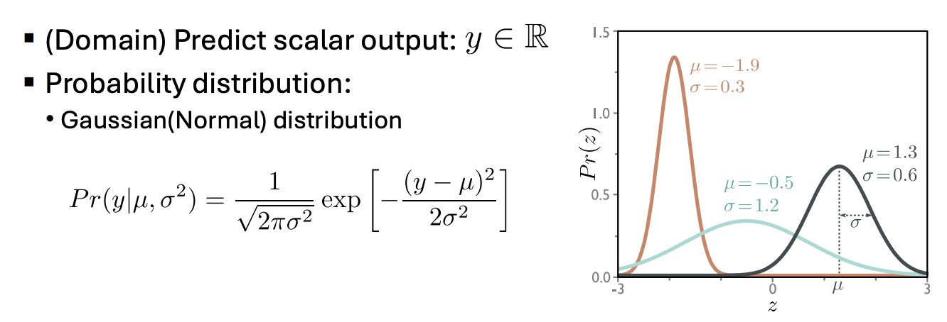
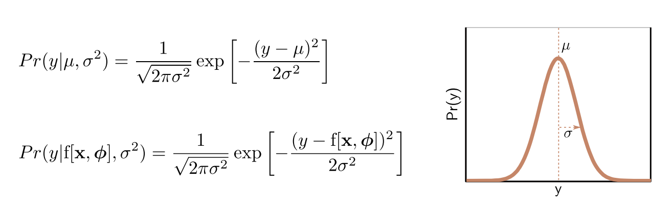
Univariate Regression

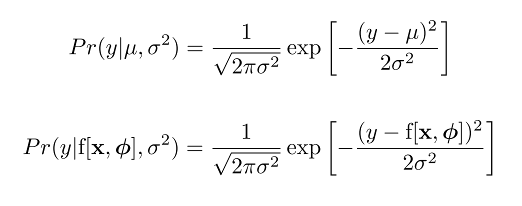
1. Choose a suitable probability distribution $Pr(y|\theta)$ defined over the domain of the predictions y with distribution parameters $\theta$.

2. Set the machine learning model $f[x, \phi]$ to predict one or more of these parameters, so $\theta = f[x, \phi]$ and $Pr(y|\theta) = Pr(y|f[x, \phi]).$

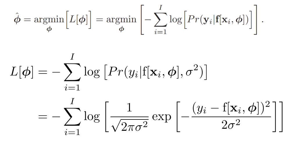
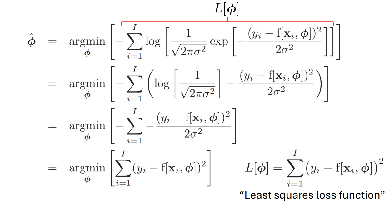
3. To train the model, find the network parameters $\hat{\phi}$ that minimize the negative log-likelihood loss function over the training dataset pairs ${x_i, y_i}$ :

4. To perform inference for a new test example x, return either the full distribution $Pr(y|f[x, \hat{\phi}]) or the value where this distribution is maximized.

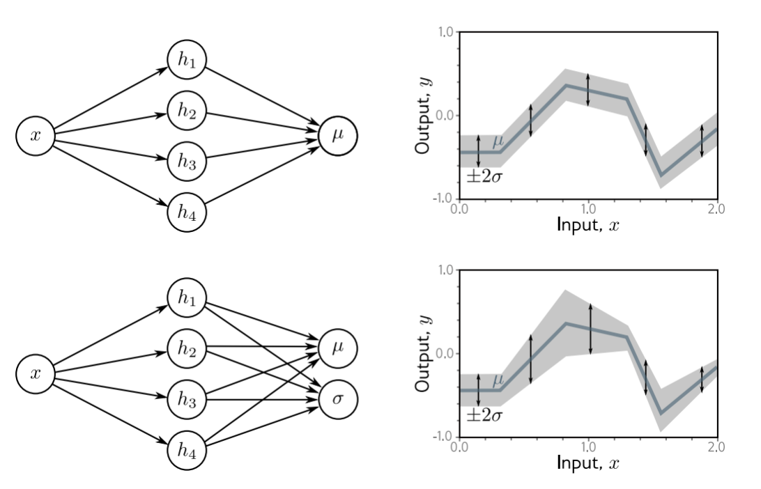
Heteroscedastic Regression

개념 요약

기존 회귀에서는 다음과 같은 가정을 한다.

$\sigma^2 = constant$

즉, 모든 데이터에서 오차 분산이 동일한 Homoscedastic 상황이다.
하지만 현실 데이터는 그렇지 않다.
입력 x에 따라 노이즈 크기가 달라지는 경우가 많다.
그래서 다음과 같이 확장한다.

$\sigma^2 = f(x)$

즉, 데이터에 따라 분산이 달라지는 회귀 모델이 바로 Heteroscedastic Regression이다.

모델 구조

이 모델은 하나의 출력이 아니라, 두 개를 동시에 예측한다.

$\mu = f_{1} (x, \phi)$

• 평균 (예측값)

  $\sigma^2 = (f_{2} (x, \phi))^2$

• 분산 (불확실성)
  핵심은 다음과 같다.

  하나의 모델이 값과 불확실성을 동시에 학습한다.

직관

기존 MSE 기반 회귀는 모든 데이터를 동일하게 본다.
하지만 이 모델은 다르다.

• 노이즈가 큰 데이터 -> 덜 신뢰
• 노이즈가 작은 데이터 -> 더 강하게 반영
  즉, 데이터마다 "신뢰도(weight)"를 다르게 두고 학습하는 방식이다.

Loss Fuction (핵심)

이 모델은 정규분포 기반 최대우도측정(MLE)을 사용한다.

$\hat{\phi} = \arg \min_{\phi} \left[ -\sum_{i=1}^{I} \log \left( \frac{1}{\sqrt{2\pi\sigma_i^2}} \right) + \frac{(y_i - \mu_i)^2}{2\sigma_i^2} \right]$

수식해석 :

$\log \frac{1}{\sqrt{2\pi\sigma^2}}$

• 분산이 크면, 패널티가 감소한다.
• 분산이 작으면, 패널티가 증가한다.
  즉, 모델이 무작성 분산을 키우지 못하게 제어한다.

오차 항 :

$\frac{(y - \mu)^2}{2\sigma^2}$

• 분산이 크면 오차 영향이 작아진다.
• 분산이 작으면 오차 영향이 커진다.

한줄 정리

Heteroscedastic Regression은 값 + 불확실성을 함께 예측하면서, 데이터별 신뢰도를 반영하는 회귀 모델이다.

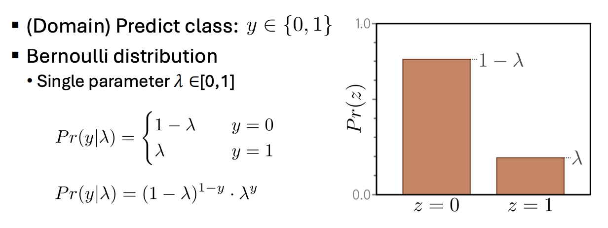
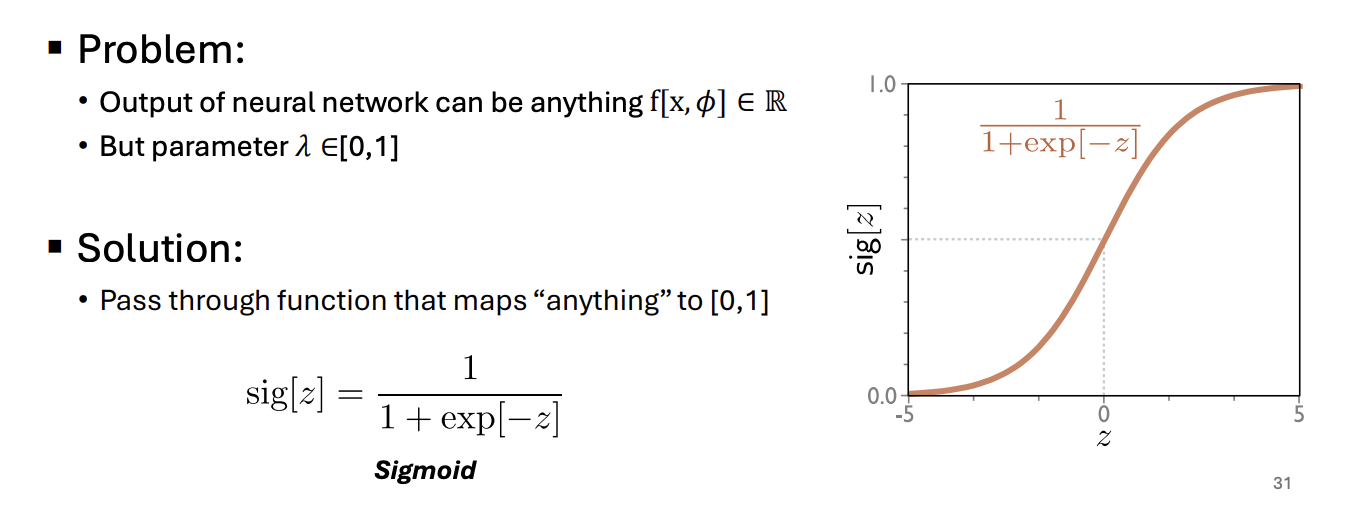
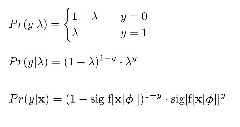
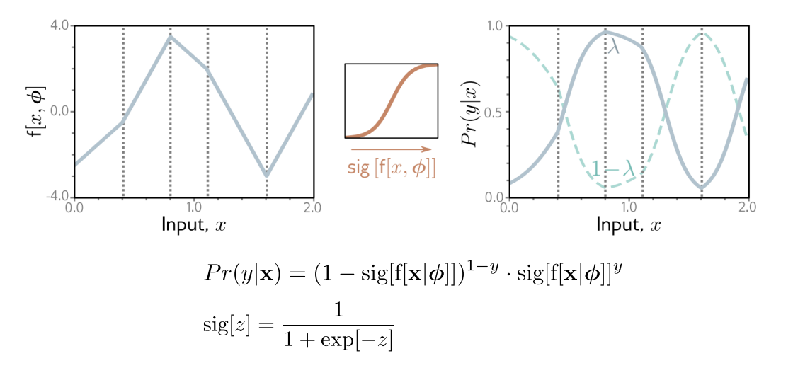
Binary Classification

1. Choose a suitable probability distribution $Pr(y|\theta)$ defined over the domain of the predictions y with distribution parameters $\theta$.

2. Set the machine learning model $f[x, \phi]$ to predict one or more of these parameters, so $\theta = f[x, \phi]$ and $Pr(y|\theta) = Pr(y|f[x, \phi]).

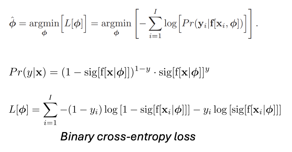
3. To train the model, find the network parameters $\hat{\phi}$ that minimize the negative log-likelihood loss function over the training dataset pairs ${x_i, y_i}$
   

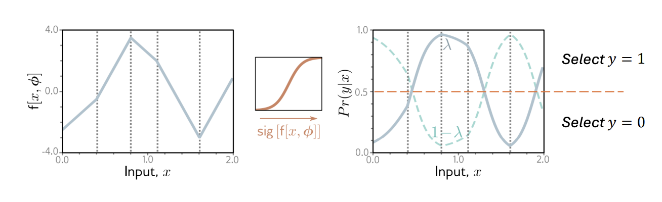
4. To perform inference for a new test example x, return either the full distribution $Pr(y|f[x, \hat{\phi}]) or the value where this distribution is maximized.

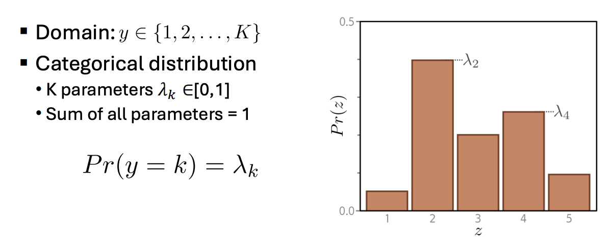
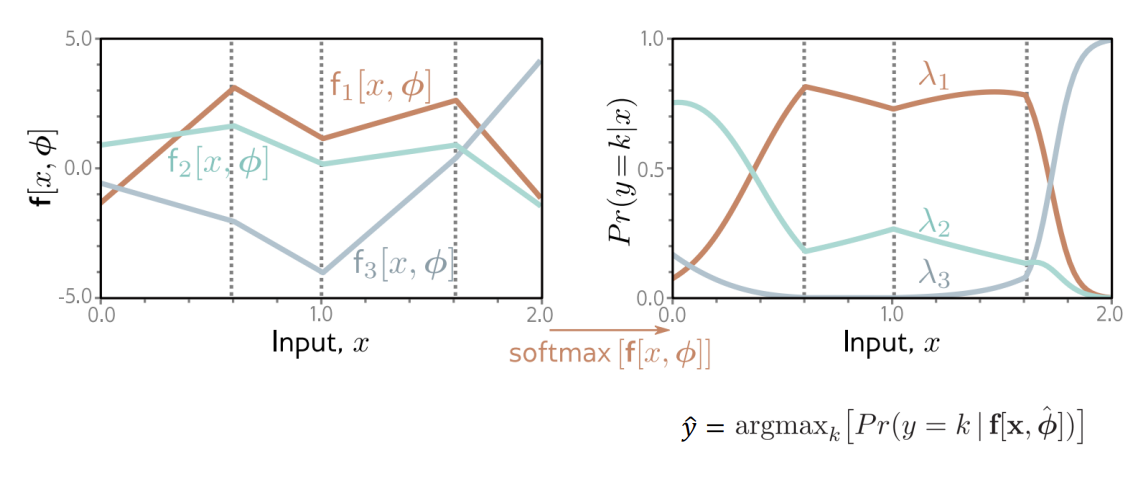
Multiclass Classification

1. Choose a suitable probability distribution $Pr(y|\theta)$ defined over the domain of the predictions y with distribution parameters $\theta$.

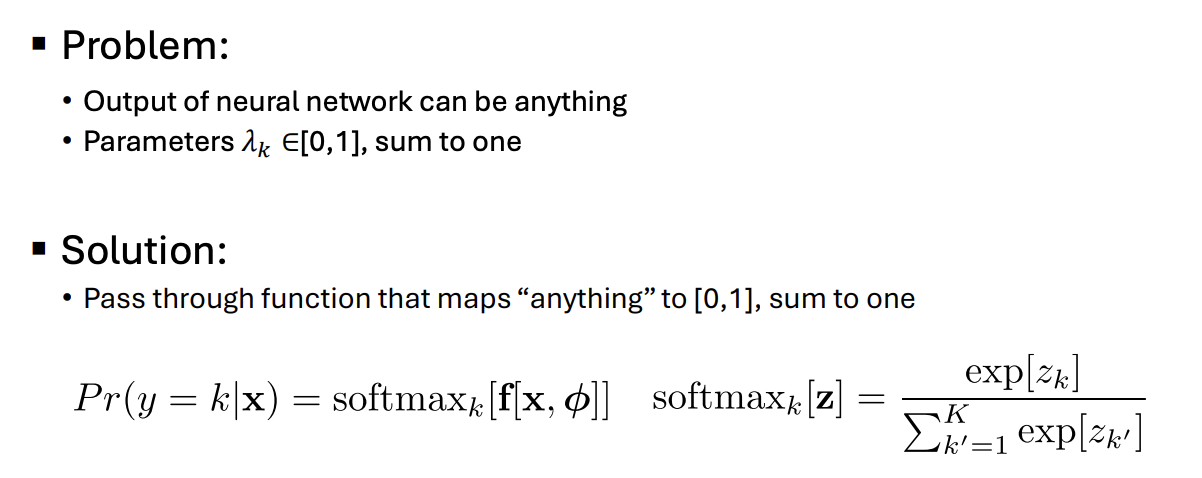
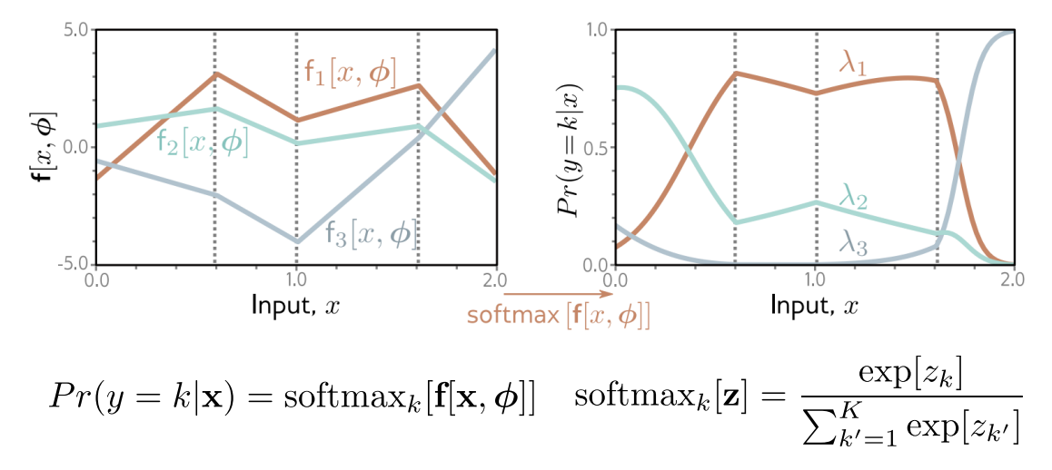
2. Set the machine learning model $f[x, \phi]$ to predict one or more of these parameters, so $\theta = f[x, \phi]$ and $Pr(y|\theta) = Pr(y|f[x, \phi]).

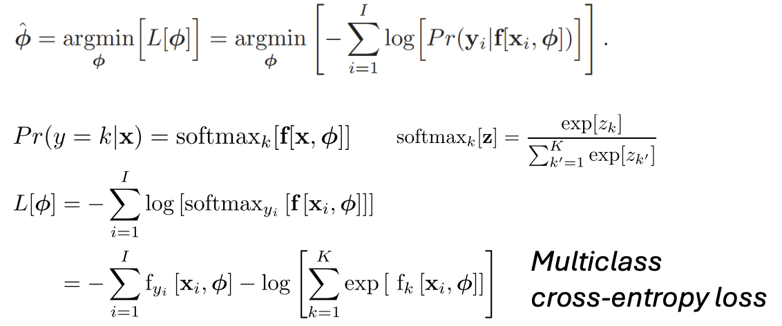
3. To train the model, find the network parameters $\hat{\phi}$ that minimize the negative log-likelihood loss function over the training dataset pairs ${x_i, y_i}$
   

4. To perform inference for a new test example x, return either the full distribution $Pr(y|f[x, \hat{\phi}]) or the value where this distribution is maximized.

Multiple Outputs (다중 출력 모델)

개념 요약

출력이 하나가 아니라 벡터인 경우를 생각해보자.

$y = (y_1, y_2, \dots, y_D)$

예:

• 좌표 예측 -> (x, y)
• 여러 타겟 -> (가격, 수요량, 위험도)

확률 분해

각 확률들은 독립이다는 가정하에, Joint Probability가 이렇게 쪼개진다.

$Pr(y | f[x_i, \phi]) = \prod_{d} Pr(y_d | f_d [x_i, \phi])$

Cross Entropy Loss & KL Divergence

핵심 개념

Cross Entropy는 사실 이것과 연결된다.

$KL(q||p)$

-> KL Eivergence (분포 간 거리)

KL Divergence 정의

$\text{KL}[q || p] = \int q(z) \log q(z) dz - \int q(z) \log p(z) dz$

의미 해석

• q(z) : 실제 데이터 분포
• p(z) : 모델이 만든 분포

KL Divergence는 모델 분포 p가 실제 분포 q와 얼마나 다른지를 보여준다.

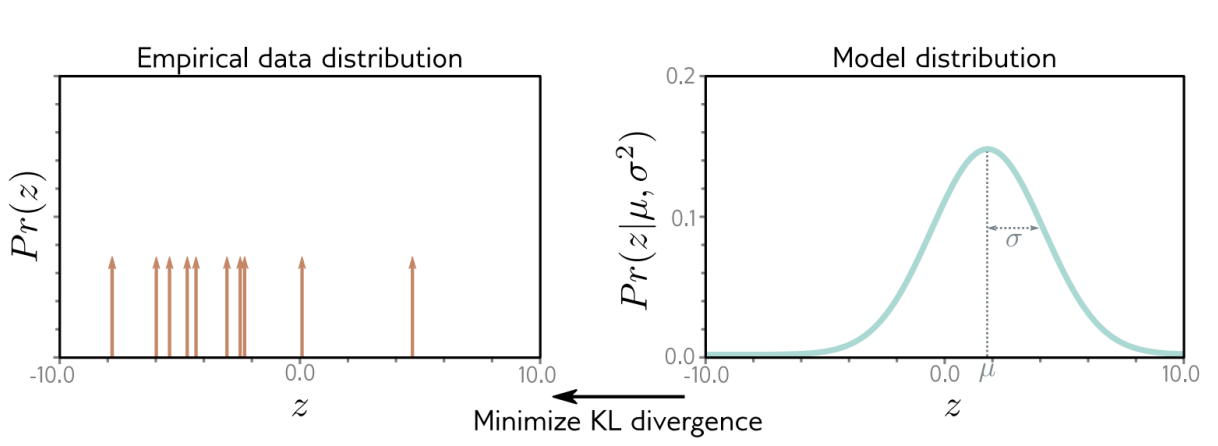
그림 직관

왼쪽 그래프는 실제 데이터 분포를 보여준다. 오른쪽은 모델이 만든 분포 Gaussian을 보여준다.

왜 Cross Entropy가 나오냐

KL식을 다시 보면,

$\text{KL}[q || p] = \int q(z) \log q(z) dz - \int q(z) \log p(z) dz$

앞에 q(z)log(q(z)는 데이터로 고정된다. 즉, 학습과 무관한 상수이다. 그래서, 우리가 실제로 최소화 하는건 뒤에 적분 식이다.

의미는 정답 분포에서 샘플 뽑아서 모델이 얼마나 잘 맞추는지를 평가한다.

Cross Entropy는 모델 분포를 실제 데이터 분포에 맞추기 위해 KL divergence를 최소화한 것이다.

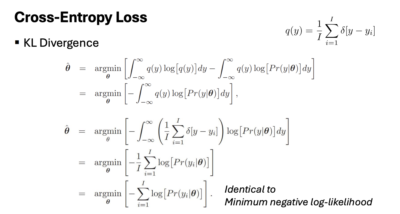
Cross Entropy를 최소화 하는것은 데이터에 대한 Likelihood를 최대화하는것과 동일하다.