이번 포스트에서는 HED (Holistically-Nested Edge Detection) 모델 구조에 대해서 알아보겠습니다.
전체 아키텍처 개요
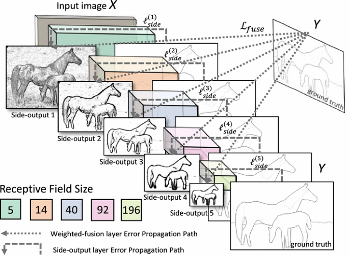
HED는 VGG-16을 백본으로 사용하는 fully convolutional network입니다. 핵심 아이디어는 deep supervision과 multi-scale feature fusion입니다.
기본 구조
Input Image (H×W×3)
    ↓
[VGG-16 Encoder with Side Outputs]
    ↓
Conv1 → Side Output 1 ─┐
Conv2 → Side Output 2 ─┤
Conv3 → Side Output 3 ─┼→ Fusion Layer → Final Edge Map
Conv4 → Side Output 4 ─┤
Conv5 → Side Output 5 ─┘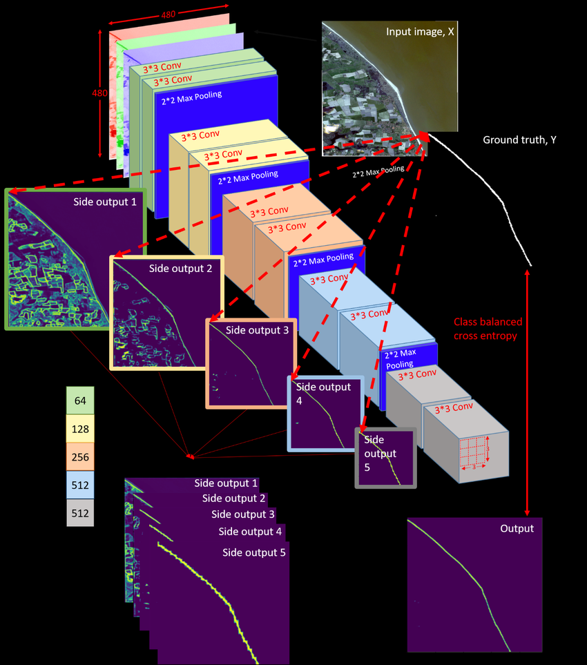
상세 구조
1. Backbone: VGG-16 기반 Encoder
Input: 224×224×3 (또는 임의 크기)

[Stage 1] - Conv1
- conv1_1: 3→64, 3×3
- conv1_2: 64→64, 3×3
- pool1: 2×2 maxpool
→ Output: 112×112×64

[Stage 2] - Conv2
- conv2_1: 64→128, 3×3
- conv2_2: 128→128, 3×3
- pool2: 2×2 maxpool
→ Output: 56×56×128

[Stage 3] - Conv3
- conv3_1: 128→256, 3×3
- conv3_2: 256→256, 3×3
- conv3_3: 256→256, 3×3
- pool3: 2×2 maxpool
→ Output: 28×28×256

[Stage 4] - Conv4
- conv4_1: 256→512, 3×3
- conv4_2: 512→512, 3×3
- conv4_3: 512→512, 3×3
- pool4: 2×2 maxpool
→ Output: 14×14×512

[Stage 5] - Conv5
- conv5_1: 512→512, 3×3
- conv5_2: 512→512, 3×3
- conv5_3: 512→512, 3×3
(pool5 없음 - HED에서는 제거)
→ Output: 14×14×512
2. Side Outputs (Deep Supervision)
각 stage의 출력마다 side output을 생성합니다:
#각 side output 구조
Side Output = 1×1 Conv → Deconv/Upsample → Sigmoid

#구체적으로:
side1: conv1_2 (112×112×64)  → 1×1 conv (64→1)  → 1×1×1     → sigmoid
side2: conv2_2 (56×56×128)   → 1×1 conv (128→1) → upsample×2 → sigmoid
side3: conv3_3 (28×28×256)   → 1×1 conv (256→1) → upsample×4 → sigmoid
side4: conv4_3 (14×14×512)   → 1×1 conv (512→1) → upsample×8 → sigmoid
side5: conv5_3 (14×14×512)   → 1×1 conv (512→1) → upsample×8 → sigmoid
모든 side output은 원본 이미지 크기로 upsampling됩니다.
3. Fusion Layer
5개의 side output을 결합:
#Concatenate along channel dimension
concat = [side1, side2, side3, side4, side5]  # Shape: H×W×5

#1×1 convolution for fusion
fuse = Conv1×1(concat, filters=1)  # 5→1
fuse = Sigmoid(fuse)  # Final edge map

##시각적 표현
224×224×3 Input
     ↓
┌────────────────────────────────────────┐
│ VGG-16 Encoder                         │
├────────────────────────────────────────┤
│ Conv1 (64 ch)  → [Side1: 1×1 conv] ───┼→ 224×224×1
│      ↓ pool                            │
│ Conv2 (128 ch) → [Side2: 1×1→up×2] ───┼→ 224×224×1
│      ↓ pool                            │
│ Conv3 (256 ch) → [Side3: 1×1→up×4] ───┼→ 224×224×1
│      ↓ pool                            │
│ Conv4 (512 ch) → [Side4: 1×1→up×8] ───┼→ 224×224×1
│      ↓ pool                            │
│ Conv5 (512 ch) → [Side5: 1×1→up×8] ───┼→ 224×224×1
└────────────────────────────────────────┘
          ↓ ↓ ↓ ↓ ↓
     [Concatenate 5 channels]
              ↓
         [1×1 Conv + Sigmoid]
              ↓
     Final Edge Map (224×224×1)
핵심 특징
- Deep Supervision
- 중간 레이어마다 직접 ground truth와 비교
- Gradient가 네트워크 전체에 효과적으로 전파
- 각 레이어가 독립적으로 edge를 학습
- Multi-Scale Feature
- Side1: 세밀한 low-level edge (텍스처, 디테일)
- Side2-3: 중간 스케일 edge
- Side4-5: 굵고 의미있는 high-level edge (객체 경계)
- Fully Convolutional
- FC layer 없음 → 임의 크기 입력 가능
- 모든 연산이 convolution → 공간 정보 보존
PyTorch 구현 예시
class HED(nn.Module):
    def __init__(self):
        super(HED, self).__init__()

        # VGG-16 backbone (pretrained 가능)
        self.conv1 = nn.Sequential(
            nn.Conv2d(3, 64, 3, padding=1),
            nn.ReLU(),
            nn.Conv2d(64, 64, 3, padding=1),
            nn.ReLU()
        )

        self.conv2 = nn.Sequential(
            nn.MaxPool2d(2, stride=2),
            nn.Conv2d(64, 128, 3, padding=1),
            nn.ReLU(),
            nn.Conv2d(128, 128, 3, padding=1),
            nn.ReLU()
        )

        # ... conv3, conv4, conv5 similar

        # Side outputs
        self.side1 = nn.Conv2d(64, 1, 1)
        self.side2 = nn.Conv2d(128, 1, 1)
        self.side3 = nn.Conv2d(256, 1, 1)
        self.side4 = nn.Conv2d(512, 1, 1)
        self.side5 = nn.Conv2d(512, 1, 1)

        # Fusion
        self.fuse = nn.Conv2d(5, 1, 1)

    def forward(self, x):
        # Encoder
        h1 = self.conv1(x)  # 224×224×64
        h2 = self.conv2(h1) # 112×112×128
        h3 = self.conv3(h2) # 56×56×256
        h4 = self.conv4(h3) # 28×28×512
        h5 = self.conv5(h4) # 14×14×512

        # Side outputs with upsampling
        s1 = torch.sigmoid(self.side1(h1))
        s2 = torch.sigmoid(F.interpolate(self.side2(h2),
                                         size=x.shape[2:],
                                         mode='bilinear'))
        s3 = torch.sigmoid(F.interpolate(self.side3(h3),
                                         size=x.shape[2:],
                                         mode='bilinear'))
        s4 = torch.sigmoid(F.interpolate(self.side4(h4),
                                         size=x.shape[2:],
                                         mode='bilinear'))
        s5 = torch.sigmoid(F.interpolate(self.side5(h5),
                                         size=x.shape[2:],
                                         mode='bilinear'))

        # Fusion
        fuse = torch.sigmoid(self.fuse(torch.cat([s1,s2,s3,s4,s5], dim=1)))

        return [s1, s2, s3, s4, s5, fuse]
VGG-16과의 차이점
- FC layer 제거: 완전 convolutional
- Pool5 제거: 해상도 유지 (일부 구현에서)
- Side outputs 추가: Deep supervision
- Fusion layer 추가: Multi-scale 결합
HED의 손실함수 구조
HED는 class-balanced cross-entropy loss를 사용합니다. 이는 edge detection에서 발생하는 심각한 클래스 불균형 문제를 해결하기 위한 것입니다.
기본 형태
각 side output에 대한 손실함수는 다음과 같습니다:
L_side = -β ∑(y=1) log P(y=1|X) - (1-β) ∑(y=0) log P(y=0|X)
여기서:
- y는 ground truth (1: edge, 0: non-edge)
- P(y|X)는 예측 확률
- β는 class-balancing weight
Class-Balancing Weight
β = |Y-| / |Y|
1-β = |Y+| / |Y|- |Y+|: edge 픽셀 수
- |Y-|: non-edge 픽셀 수
- |Y|: 전체 픽셀 수
-> 일반적인 이미지에서 edge 픽셀은 전체의 5% 미만입니다. 가중치 없이 학습하면 모델이 모든 픽셀을 non-edge로 예측해도 95% 정확도를 얻게 되어 제대로 학습되지 않습니다.
전체 손실함수
HED는 여러 side output을 가지므로:
L_total = ∑(m=1 to M) α_m × L_side^(m) + L_fuse
- M: side output 개수 (보통 5개)
- α_m: 각 side output의 가중치 (논문에서는 모두 1로 설정)
- L_fuse: 최종 fused output의 손실
각 side output과 최종 fusion output 모두 동일한 ground truth와 비교하여 학습됩니다.
loss 함수 구현
def hed_loss(predictions, targets):
    """
    predictions: [batch, 1, H, W] - sigmoid 출력
    targets: [batch, 1, H, W] - binary ground truth
    """
    # Class balancing weight 계산
    pos_pixels = torch.sum(targets == 1).float()
    neg_pixels = torch.sum(targets == 0).float()
    total_pixels = pos_pixels + neg_pixels

    beta = neg_pixels / total_pixels  # non-edge 비율

    # Class-balanced cross entropy
    loss = -beta * targets * torch.log(predictions + 1e-8) \
           - (1 - beta) * (1 - targets) * torch.log(1 - predictions + 1e-8)

    return torch.mean(loss)

# 전체 손실 (5개 side output + 1개 fuse)
total_loss = sum([hed_loss(side_out, gt) for side_out in side_outputs]) \
             + hed_loss(fuse_output, gt)
따라가기도 벅찬 AI Engineer 겸 부앙단