Proximal Policy Optimization

Roh's warehouse·2025년 9월 22일

Introduction to RL

목록 보기

10/10

최근 가장 많이 사용되는 policy-based RL 알고리즘으로는 proximal policy optimization (PPO)이 있다. PPO는 trust region policy optimization (TRPO) 알고리즘으로부터 유도되었기에 PPO를 설명하기 전 우선 TRPO에 대해서 설명한다.

Trust Region Policy Optimization (TRPO)

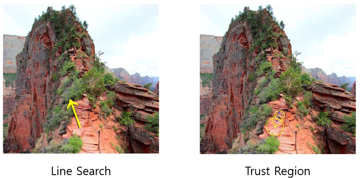
Line Search vs. Trust Region

만약 우리가 산 정상을 향해 올라가는 길을 탐색한다고 하자.

Line search는 (가장) 가파른 방향을 선택하고 정해진 간격만큼 그 방향으로 이동하는 것이다. 우리가 주로 사용하는 gradient descent가 이에 해당한다. 만약 이동 간격이 너무 작다면, 정상에 도달하는데 너무 오랜 시간이 소요될 것이고, 간격이 너무 크다면 절벽으로 떨어질 수 있다.

Trust region을 이용한 방법은 우선 우리가 탐색할만큼의 이동 간격을 설정하고, 해당 구간 (아래 그림에서 노란 원)에서 새로운 optimal point를 찾아 그 공간으로 이동하는 것이다. 이 과정을 반벅하면 보다 안정적으로 정상에 도달할 수 있다. 하지만, trust region 방법은 line search에 비해 높은 계산량을 요구한다는 단점이 있다.

Problem Definition of TRPO

TRPO는 기본적으로 policy update 과정에서 trust region 방식을 사용한다. 이 때, 이동 간격이 너무 커지지 않도록 constraint를 설정한다. 이 constraint는 old policy와 new policy의 분포가 너무 달라지지 않도록하는 역할을 하며, 이를 위해 KL-divergence를 통해 제약을 설정한다.

그 동안의 policy gradient 알고리즘들의 경우, old policy와 new policy의 분포가 아닌, parameter space에서의 거리에 대한 제한을 두었다고 볼 수 있다. 하지만, parameter space에서의 작은 차이가 실제 policy 분포에서는 큰 차이를 유발할 수 있기 때문에 policy의 convergence에서의 문제가 있었다.

TRPO 문제를 수리적으로 정의하면 다음과 같다.

\max \, J(\theta, \theta_{\text{old}}) \quad \text{s.t.} \quad \overline{KL}(\theta, \theta_{\text{old}}) \leq \delta

여기서, $J(\theta, \theta_{\text{old}})$ 와 $\overline{KL}(\theta, \theta_{\text{old}})$ 은 다음과 같이 정의된다.

J(\theta, \theta_{\text{old}}) = \mathbb{E}_{\pi_\theta} \left[ \frac{\pi_\theta(a \mid s)}{\pi_{\theta_{\text{old}}}(a \mid s)} A^{\pi_{\theta_{\text{old}}}}(s, a) \right]

\overline{KL}(\theta, \theta_{\text{old}}) = \mathbb{E}_{\pi_\theta} \left[ KL(\pi_{\theta_{\text{old}}}(\cdot \mid s), \pi_\theta(\cdot \mid s)) \right]

TRPO는 old policy에 기반하여 new policy의 performance를 maximize한다. 수리적으로 보면, TRPO의 objective는 new policy에 대한 advantage function의 기댓값이다. 다만, 여기서의 advantage function $A$ 는 old policy를 통해 estimate 된 값으로, $\frac{\pi_\theta(a \mid s)}{\pi_{\theta_{\text{old}}}(a \mid s)}$ 를 이용해 new policy의 값으로 조정된다.

Objective의 경우 old policy와 new policy의 차이가 클수록 조정의 정확도가 떨어진다.

TRPO의 constraint는 old/new policy간의 KL-divergence에 대한 크기 제한( $\delta$ )을 통해 new policy가 너무 크게 변화하는 것을 방지한다.

TRPO는 old policy의 data만을 사용하기 때문에 on-policy algorithm이 된다.

TRPO Solution

$J(\theta, \theta_{\text{old}})$ 에 Talyer expansion at $\theta_{\text{old}}$ 을 적용해보자.

J(\theta, \theta_{\text{old}}) \approx J(\theta_{\text{old}}, \theta_{\text{old}}) + g^T(\theta - \theta_{\text{old}}) + \cdots

여기서 $g = \nabla_\theta J(\theta, \theta_{\text{old}}) \mid_{\theta_{\text{old}}}$ 로, $J$ 의 gradient 값을 말한다.

이 때, $J(\theta_{\text{old}}, \theta_{\text{old}})$ 는 constant 값이기에 maximization에 영향을 끼치지 않는다. 또한, higher-order term은 무시할 수 있다고 하자. 이 경우, objective를 다음과 같이 쓸 수 있다.

J(\theta, \theta_{\text{old}}) \approx g^T(\theta - \theta_{\text{old}})

추가로, constraint $\overline{KL}(\theta, \theta_{\text{old}})$ 에 Talyer expansion at $\theta_{\text{old}}$ 을 적용하면 다음 식을 얻을 수 있다.

\overline{KL}(\theta, \theta_{\text{old}}) \approx \overline{KL}(\theta_{\text{old}}, \theta_{\text{old}}) + \nabla_\theta \overline{KL}(\theta, \theta_{\text{old}}) \mid_{\theta_{\text{old}}} (\theta - \theta_{\text{old}})

+ \frac{1}{2} (\theta - \theta_{\text{old}})^T H (\theta - \theta_{\text{old}}) + \cdots

여기서 $H = \nabla_\theta^2 \overline{KL}(\theta, \theta_{\text{old}}) \mid_{\theta_{\text{old}}}$ 로, $\overline{KL}$ 의 Hessian 값을 말한다.

이 때, $\overline{KL}(\theta_{\text{old}}, \theta_{\text{old}}) = 0$ 이다. 또한, $\nabla_\theta \overline{KL}(\theta, \theta_{\text{old}}) \mid_{\theta_{\text{old}}}=0$ 이 알려져 있다.

따라서, constraint를 다음과 같이 쓸 수 있다.

\overline{KL}(\theta, \theta_{\text{old}}) \approx \frac{1}{2} (\theta - \theta_{\text{old}})^T H (\theta - \theta_{\text{old}})

위 내용을 토대로 TRPO 문제를 다음과 같이 표현할 수 있다.

\begin{aligned} \max_\theta \quad &g^T(\theta - \theta_{\text{old}}) \\ \text{s.t.} \quad &(\theta - \theta_{\text{old}})^T H (\theta - \theta_{\text{old}}) \leq \delta \end{aligned}

Analytic Solution of TRPO

새롭게 정의된 위 TRPO 문제에 대해 Taylor expansion을 이용한 approximate solution을 다음 recurrent equation을 통해 표현할 수 있다.

\theta_{k+1} = \theta_k + \sqrt{\frac{2\delta}{g^T H^{-1} g}} H^{-1} g

위 solution은 approximate solution이기에 KL constraint를 위반할 수 있고, objective를 maximize하지 않을 수도 있다.

위 식을 이용해 line search를 통한 update가 가능하다.

\theta_{k+1} = \theta_k + \alpha^j\sqrt{\frac{2\delta}{g^T H^{-1} g}} H^{-1} g

여기서 $\alpha \in (0,1)$ 은 backtracking coefficient, $j$ 는 KL constraint를 만족하면서 positive objective를 만드는 최소한의 양의 정수를 말한다.

하지만, 역행렬 $H^{-1}$ 의 계산 비용은 무척 높은 관계로 위 방법은 거의 사용되지 않는다.

Issue of TRPO

따라서, TRPO 문제를 해결하는 또 다른 방법은 Lagrange multiplier $\lambda$ 를 이용하는 것이다.

\max \, \mathbb{E}_{\pi_\theta} \left[ \frac{\pi_\theta(a \mid s)}{\pi_{\theta_{\text{old}}}(a \mid s)} A^{\pi_{\theta_{\text{old}}}}(s, a) - \lambda KL(\pi_{\theta_{\text{old}}}(\cdot \mid s), \pi_\theta(\cdot \mid s)) \right]

이러한 방식은, constraint를 penalty로 전환하는 것으로, 이론적인 관점에서는 다루기가 더 쉽기 때문에 좋게 볼 수도 있다. 하지만, 실제로는 하나의 $\lambda$ (penalty term)을 선택하는 것은 무척 어렵다. 이는 문제마다 다르고, 또 하나의 문제 내에서 최적의 $\lambda$ 값은 학습을 진행함에 따라 바뀌기 때문이다.

따라서, 이러한 TRPO의 계산적 어려움을 극복할 수 있는 개선된 방법이 요구되었다.

Proximal Policy Optimization (PPO)

PPO는 TRPO의 계산적 어려움을 개선한 알고리즘이다. 두 알고리즘은 policy의 급격한 변화를 방지하면서 policy에 대한 개선을 진행한다는 점에서 같은 목적을 갖는다. 하지만, TRPO는 복잡한 second-order optimization을 사용하는 반면, PPO는 몇 가지 trick을 가미한 first-order method를 사용하기 때문에 훨씬 쉽게 구현이 가능하면서도, 더 나은 성능을 보여준다.

PPO는 크게 PPO-clip과 PPO-penalty으로 나눌 수 있다. PPO-clip은 constraint가 없이, objective에 clipping을 적용하여 new policy가 old policy로부터 너무 멀어지는 것을 방지한다. PPO-penalty는 앞서 서술한 unconstraint problem에서 penalty term $\lambda$ 를 학습을 진행하면서 자동으로 조정하여 풀어내는 방법이다.

PPO-Clip

PPO-clip의 경우, 다음과 같이 쓸 수 있다:

\max \, \mathbb{E}_{\pi_\theta} \left[ J_{\text{PPO}} \right]

where,

J_{\text{PPO}} = \min \left( \frac{\pi_\theta(a \mid s)}{\pi_{\theta_{\text{old}}}(a \mid s)} A^{\pi_{\theta_{\text{old}}}}(s, a), \, \text{clip} \left( \frac{\pi_\theta(a \mid s)}{\pi_{\theta_{\text{old}}}(a \mid s)}, \, 1 - \epsilon, \, 1 + \epsilon \right) A^{\pi_{\theta_{\text{old}}}}(s, a) \right).

여기서 $\epsilon$ 은 clipping의 정도를 결정하는 hyperparameter로, policy의 ratio가 $(1-\epsilon, 1+\epsilon)$ 으로 제한되도록 강제한다.

만약, advantage $A$ 가 positive한 경우, $J_{\text{PPO}}$ 는 다음과 같다.

J_{\text{PPO}} = \min \left( \frac{\pi_\theta(a \mid s)}{\pi_{\theta_{\text{old}}}(a \mid s)}, \, 1 + \epsilon \right) A^{\pi_{\theta_{\text{old}}}}(s, a)

반대로, advantage $A$ 가 negative한 경우, $J_{\text{PPO}}$ 는 다음과 같다.

J_{\text{PPO}} = \max \left( \frac{\pi_\theta(a \mid s)}{\pi_{\theta_{\text{old}}}(a \mid s)}, \, 1 - \epsilon \right) A^{\pi_{\theta_{\text{old}}}}(s, a)

이러한 clipping 방법은 일종의 regularization의 효과를 갖는다.

일반적으로 $\epsilon=0.2$ 일 때 좋은 성능을 보여준다.

PPO-Penalty

PPO-penalty는 policy update를 진행할 때마다 penalty coefficient를 수정하며 최적화를 진행한다.

일반적으로 PPO-penalty가 PPO-clip보다 성능이 좋지 않다는 것이 알려져 있다.

즉, 아래 식을 optimize한다.

J_{\text{KLPEN}} = \mathbb{E}_{\pi_\theta} \left[ \frac{\pi_\theta(a \mid s)}{\pi_{\theta_{\text{old}}}(a \mid s)} A^{\pi_{\theta_{\text{old}}}}(s, a) - \lambda KL(\pi_{\theta_{\text{old}}}(\cdot \mid s), \pi_\theta(\cdot \mid s)) \right]

이 때, 매 update마다 아래 식을 통해 $\lambda$ 를 조정한다.

d = KL(\pi_{\theta_{\text{old}}}(\cdot \mid s), \pi_\theta(\cdot \mid s))

\begin{cases} \lambda \leftarrow \lambda / 2 & \text{if} \quad d < d_{\text{targ}} / 1.5 \\ \lambda \leftarrow \lambda \times 2 & \text{if} \quad d > d_{\text{targ}} \times 1.5 \end{cases}

여기서 $d_{\text{targ}}$ 은 KL divergence의 target value이다.

Summary of PPO

PPO는 간단한 수식을 갖고 있음에도 가장 훌륭한 성능을 보여주는 policy gradient method이다. 기존의 vanilla PG 방법들이 data efficiency 및 robustness 측면에서 좋지 않은 성능을 보여주었고, 개선된 방법인 TRPO는 로직이 복잡하고 학습이 어렵다는 단점을 가지고 있었다. PPO는 이러한 단점을 모두 극복한 로직으로 가장 널리 사용되는 알고리즘이다.

PPO를 제외하고도 DDPG 및 SAC 등 다양한 policy-based RL 알고리즘들이 존재하니, 이를 참고해보자.