잡담
너무 힘들다ㅠㅠ 지금까지처럼, 포기하지않고 열심히 하면 언젠가 보상받는 날이 오겠지? 비록 20대만큼의 액티브한 인생은 아니지만, 30대의 또 하나의 거대한 목표를 이루기위해 열심히 달리자. 아자아자 !
영어로 말하기(완료)많은 나라 돌아다니기(완료)- 한 분야의 전문가 되기 (진행 중)
- We are the One ! (언젠가 시작하겠지 ㅋㅋㅋ)
실습 코드
모델 성능 검증 방법(Holdout / K-Fold Cross Validation / LOOCV)을 실제 모델에 적용해보자.
공부를 위해 직접 구현된 코드를 활용하여, 모델의 성능을 확인한다.
예측 모델 정의
Age에 대해 Height를 예측하는 선형 기저 함수 모델을 생성 한다.
데이터 생성
- x = Age
- T = Height
import numpy as np
import matplotlib.pyplot as plt
%matplotlib inline

np.random.seed(seed=1)
x_min = 4  # 최소
x_max = 30 # 최대
x_n = 16  # 데이터 수

x = 5 + 25 * np.random.rand(x_n)

Prm_c = [170, 108, 0.2]
T = Prm_c[0] - Prm_c[1] * np.exp(-Prm_c[2] * x) + 4 * np.random.randn(x_n)

# 데이터 로드
np.savez('ch5_data.npz', x=x, x_min=x_min, x_max=x_max, x_n = x_n, T=T)
outfile = np.load('/content/ch5_data.npz')

x = outfile['x']
x_min = outfile['x_min']
x_max = outfile['x_max']
x_n = outfile['x_n']
T = outfile['T']
모델 함수 정의
def gauss(x, mu, s):
  return np.exp(-(x-mu)**2 / (2*s**2))
선형 기저 함수 모델
# 선형 기저 함수 모델
def gauss_func(w, x):
  m = len(w) - 1
  mu = np.linspace(5, 30, m) # 평균값
  s = mu[1] - mu[0] # 분산
  y = np.zeros_like(x) # x와 같은 크기로 요소와 0의 행렬 y 작성

  for j in range(m):
    y = y + w[j] * gauss(x, mu[j], s)


  y = y + w[m]

  return y
가우스함수의 MSE 구하기
def mse_gauss_func(x,t,w):
  y = gauss_func(w, x)
  mse = np.mean((y-t)**2)
  return mse
가우스 함수 해석해를 통해 가중치(w) 구하기
# 선형기저 함수 모델의 해석해
def fit_gauss_func(x,t,m):
  mu = np.linspace(5, 30, m) # linspace(start, stop, number of value in array)
  s = mu[1] - mu[0]
  n = x.shape[0] # x.shape = (16)
  phi = np.ones((n, m +1)) # m+1은 마지막 Bias 고려한 숫자

  for j in range(m):
    phi[:, j] = gauss(x, mu[j], s) # [phi_j0, phi_j1, phi_j2, phi_j3] | m = 4

  phi_T = np.transpose(phi)

  b = np.linalg.inv(phi_T.dot(phi))
  c = b.dot(phi_T)
  w = c.dot(t)

  return w
그래프 그리기
# Gauss Basus Function을 그래프에 Drawing
def show_gauss_func(w):
    xb = np.linspace(x_min, x_max, 100)
    y = gauss_func(w, xb)
    plt.plot(xb, y, c=[.5, .5, .5], lw=4)
검증
Holdout
훈련 데이터: 전체 데이터의 3/4, 테스트 데이터 1/4
# Split the feature vector "X" into Test (1/4) and Training dataset (3/4).
x_test = x[ :int(x_n / 4)]
x_training = x[int(x_n / 4): ]
print("x_test.shape: {}".format(x_test.shape),"x_training.shape: {}".format(x_training.shape))
# Split the feature vector "T" into Test (1/4) and Training dataset (3/4).
t_test = T[ :int(x_n / 4)]
t_training = T[int(x_n / 4): ]
print("y_test.shape: {}".format(t_test.shape),"y_training.shape: {}".format(t_training.shape))
Print 결과로, Test / Training Data가 4:1 로 나누어졌다.
x_test.shape: (4,) x_training.shape: (12,)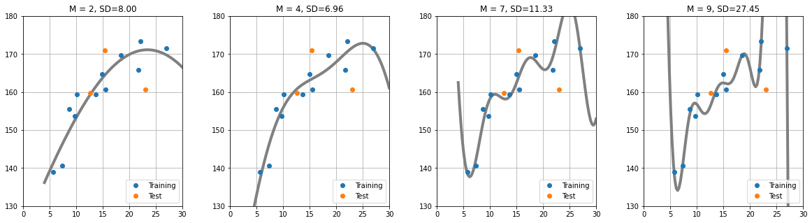
y_test.shape: (4,) y_training.shape: (12,)(사용하는 가우스 함수 개수)의 개수에 대해, 외부 데이터(Test)의 성능(SD,MSE)을 살펴보자.
plt.figure(figsize=(20,5))

plt.subplots_adjust(wspace = 0.3) # subplot 간격

M = [2, 4, 7, 9] # 가우스 함수의 개수

for i in range(len(M)):
  plt.subplot(1, len(M), i+1)
  w = fit_gauss_func(x_training, t_training, M[i])
  show_gauss_func(w) # Training Data로 구한 가중치를 사용하여 W 계산
  plt.plot(x_training, t_training, marker='o', linestyle='None', label = 'Training') # X to T data plot for Training
  plt.plot(x_test, t_test, marker='o', linestyle='None', label = 'Test') # X to T data plot for Test
  plt.legend(loc = 'lower right')
  plt.xlim(0, x_max)
  plt.ylim(130, 180)
  plt.grid(True)
  mse = mse_gauss_func(x_test, t_test, w) # 학습된 모델에서, Test 데이터로 MSE 계산
  plt.title("M = {0:d}, SD={1:.2f}".format(M[i], np.sqrt(mse)))
출력시, M=4 일때 테스트 데이터 x_test의 예측결과 성능이 가장 뛰어나다. M=7 or 9 일때 그래프 추세를 보면 데이터에 대한 오버피팅이 일어나, x_test 데이터에 대해 예측성능이 낮은것으로 관측된다.

K-Fold Cross Validation
1/4 의 데이터를 테스트용으로만 사용하고 버리는것은 낭비다. 모든 데이터를 K개의 그룹으로 나누어 모델을 K개 생성하여 성능을 평가해보자.
k개의 그룹 생성 및 Test / Training 데이터로 분리하는 함수 생성
# K겹 교차 검증

def kfold_gauss_func(x,t,m,k):
    n = x.shape[0]
    mse_train = np.zeros(k) # k 개의 모델 생성
    mse_test = np.zeros(k)

    for i in range(0, k):
        x_train = x[np.fmod(range(n), k) != i] # Boolean Slicing
        t_train = t[np.fmod(range(n), k) != i]
        x_test = x[np.fmod(range(n), k) == i]
        t_test = t[np.fmod(range(n), k) == i]
        # np.fmod(n,k): n을 k로 나누었을때, 나머지 출력
        # n을 range(n)으로 하면, 0 ~ (k-1) 까지 반복 가능.
        wm = fit_gauss_func(x_train, t_train, m)
        mse_train[i] = mse_gauss_func(x_train, t_train, wm)
        mse_test[i] = mse_gauss_func(x_test, t_test, wm)

    return mse_train, mse_test
Training / Test 데이터의 MSE 비교
# Training 데이터의 MSE와, Test 데이터의 MSE 비교
M = 4
K = 4
mse_train, mse_test = kfold_gauss_func(x,T,M,K)
print("Training:",mse_train,"\nTest:",mse_test) Training: [12.87927851 9.81768697 17.2615696 12.92270498]
Test: [ 39.65348229 734.70782018 18.30921743 47.52459642]LOOCV (Leave One Out Cross Validation)
사용하는 데이터셋의 개수가 16개 밖에 없음으로, 일반적인 K겹 교차 검증보다, 테스트 데이터 샘플을 하나만 사용하는 LOOCV로 모델의 성능을 평가해보자.
## LOOCV: K겹 교차검증의 한 종류로, 테스트 데이터를 단 하나의 샘플데이터만 사용

M = range(2,8)
k = 16 # 생서 모델 16개

cv_gauss_train = np.zeros((k, len(M)))
cv_gauss_test = np.zeros((k,len(M)))

for i in range(0, len(M)):
  cv_gauss_train[:, i], cv_gauss_test[:, i] = kfold_gauss_func(x, T, M[i], k) # Return mse_train, mse_test
  mean_gauss_train = np.sqrt(np.mean(cv_gauss_train, axis = 0)) # axis=0 각 세로열에 대한 평균 계산: https://numpy.org/doc/stable/reference/generated/numpy.mean.html
  print("Training: ",mean_gauss_train)
  mean_gauss_test = np.sqrt(np.mean(cv_gauss_test, axis=0))
  print("    Test: ",mean_gauss_test)
  print("========="*10)

# print(cv_gauss_train)
# print("========="*10)
# print(cv_gauss_test)
Training: [4.61635046 0. 0. 0. 0. 0. ]
Test: [6.79878801 0. 0. 0. 0. 0. ]
==========================================================================================
Training: [4.61635046 4.30457318 0. 0. 0. 0. ]
Test: [6.79878801 6.51404221 0. 0. 0. 0. ]
==========================================================================================
Training: [4.61635046 4.30457318 3.88914576 0. 0. 0. ]
Test: [ 6.79878801 6.51404221 13.01993566 0. 0. 0. ]
==========================================================================================
Training: [4.61635046 4.30457318 3.88914576 3.67542755 0. 0. ]
Test: [ 6.79878801 6.51404221 13.01993566 16.05453582 0. 0. ]
==========================================================================================
Training: [4.61635046 4.30457318 3.88914576 3.67542755 3.32505819 0. ]
Test: [ 6.79878801 6.51404221 13.01993566 16.05453582 17.36285834 0. ]
==========================================================================================
Training: [4.61635046 4.30457318 3.88914576 3.67542755 3.32505819 3.27188164]
Test: [ 6.79878801 6.51404221 13.01993566 16.05453582 17.36285834 45.59312959]
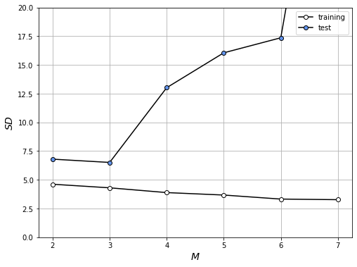
==========================================================================================M에 대한 SD(모델의 성능 평가지표)를 가시적으로 확인해 보자.
plt.figure(figsize=(8,6))
plt.plot(M, mean_gauss_train, marker = 'o', linestyle = '-', color = 'k', markerfacecolor = 'w', label = 'training')
plt.plot(M, mean_gauss_test, marker = 'o', linestyle='-', color='k', markerfacecolor = 'cornflowerblue', label='test')
plt.legend(loc="upper_left", fontsize=10)
plt.xlabel("$M$", fontsize=14)
plt.ylabel("$SD$", fontsize=14)
plt.ylim(0,20)
plt.grid(True)
plt.show()
LOOCV로 모델의 성능을 평가 했을때, M=3일때의 SD가 가장 낮다.
M=3일때의 예측모델을 생성해보자.
M = 3
plt.figure(figsize = (4, 4))
W = fit_gauss_func(x, T, M)
show_gauss_func(W)
plt.plot(x, T, marker = 'o', linestyle = 'none', color = 'cornflowerblue', markeredgecolor = 'black')
plt.xlim([x_min, x_max])
plt.xlabel('age $x$')
plt.ylabel('height $t$')
plt.grid(True)
mse = mse_gauss_func(x, T, W)

plt.title("SD= {0:.2f} cm" .format(np.sqrt(mse)))
plt.show()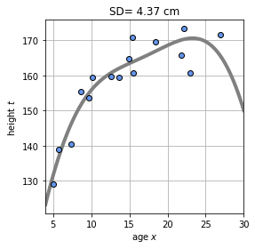
이렇게, 다양한 검증방법을 통해 여러 모델의 성능을 테스트 해보았다.
LOOCV 라이브러리 활용하기
sklearn에서 제공하는 라이브러 LeaveOneOut을 사용하여, 동일한 실습파일에 대한 성능을 추정해보자.
- modele_selection으로 부터
LeaveOneOut라이브러리 호출
import numpy as np
from sklearn.model_selection import LeaveOneOut- 인스턴스하기
loo = LeaveOneOut()
loo.get_n_splits(x) # Returns 16 as the number of dataset are 16. - Test / Train 데이터 분리
M = range(2,8) # 2,3,4,5,6,7
k = 16 # 생서 모델 16개
mse_train = np.zeros((k,len(M))) # 16(k) * 6(M)
mse_test = np.zeros((k,len(M)))
for train_index, test_index in loo.split(x):
print("===="*20)
print("Train Index: {}".format(train_index), "\nTest Index: {}".format(test_index))
print("===="*20)
x_train, x_test = x[train_index], x[test_index]
t_train, t_test = T[train_index], T[test_index]
print("X_Train: \n", x_train, "\nX_Test:", x_test, "\nT_Train: \n", T_train, "\nT_Test:", T_test)
for i in range(0, len(M)):
w_train = fit_gauss_func(x_train, t_train, M[i]) # M[0]=2, M[1], M[2], M[3], M[4], M[5]에 대한 w_train 값을 반환 후 저장
mse_train[int(test_index),i] = mse_gauss_func(x_train,t_train, w_train)
mse_test[int(test_index),i] = mse_gauss_func(x_test,t_test, w_train)
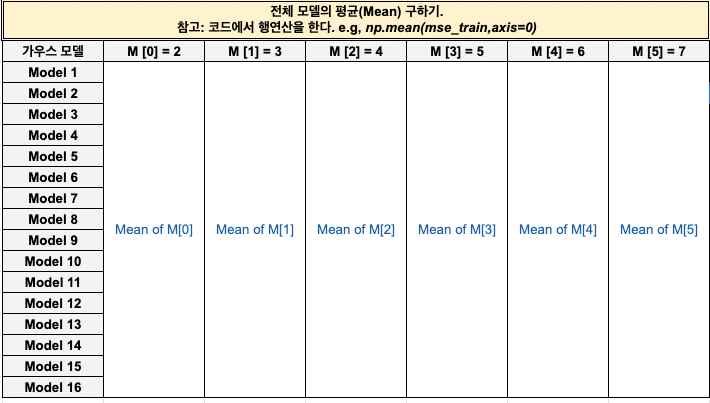
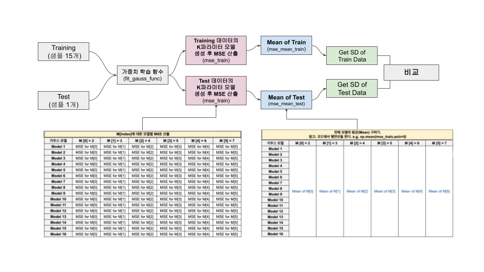
mse_mean_train = np.mean(mse_train,axis=0) # axis가 0 일때, row를 기준으로 mean 값 추출
mse_mean_test = np.mean(mse_test,axis=0)
mean_sd_train = np.sqrt(mse_mean_train)
mean_sd_test = np.sqrt(mse_mean_test) a. loo.split(x) 는 Train과 Test의 인덱스를 리턴
b. mse_train / mse_test 는 16개 (K=16)의 모델을 생성 하여 MSE값을 저장한다. M의 개수에 대한, MSE 값을 구해야하기때문에 Column은 6개가 된다.
c. 각 M에 대한 w_train을 구하고, Test / Train 데이터에 대한 가우스 함수를 구한다(mse_gauss_func)
d. mse_train[int(test_index),i]는 Column (0 to 5)에 MSE값을 저장하고 for문을 새로 돌때마다 다음 Row에 새로운 모델의 MSE를 저장한다.
e. np.mean(mse_test, axis=0)는 모델의 전체적인 성능을 평가하기 위해, 평균을 계산한다. axis=0은 row를 기준으로 평균을 계산한다. 아래 이미지를 참고하자.
모델 평가 절차를 눈으로 확인해보자.
================================================================================
Train Index: [ 1  2  3  4  5  6  7  8  9 10 11 12 13 14 15]
Test Index: [0]
================================================================================
X_Train:
 [23.00811234  5.00285937 12.55831432  8.66889727  7.30846487  9.65650528
 13.63901818 14.91918686 18.47041835 15.47986286 22.13048751 10.11130624
 26.95293591  5.68468983 21.76168775]
X_Test: [15.42555012]
T_Train:
 [170.91013145 160.67559882 129.00206616 159.70139552 155.46058905
 140.56134369 153.65466385 159.42939554 164.70423898 169.64527574
 160.71257522 173.28709855 159.31193249 171.51757345 138.9570433 ]
T_Test: [165.8744074]
================================================================================
Train Index: [ 0  2  3  4  5  6  7  8  9 10 11 12 13 14 15]
Test Index: [1]
================================================================================
X_Train:
 [15.42555012  5.00285937 12.55831432  8.66889727  7.30846487  9.65650528
 13.63901818 14.91918686 18.47041835 15.47986286 22.13048751 10.11130624
 26.95293591  5.68468983 21.76168775]
X_Test: [23.00811234]
T_Train:
 [170.91013145 160.67559882 129.00206616 159.70139552 155.46058905
 140.56134369 153.65466385 159.42939554 164.70423898 169.64527574
 160.71257522 173.28709855 159.31193249 171.51757345 138.9570433 ]
T_Test: [165.8744074]
================================================================================
Train Index: [ 0  1  3  4  5  6  7  8  9 10 11 12 13 14 15]
Test Index: [2]
================================================================================
X_Train:
 [15.42555012 23.00811234 12.55831432  8.66889727  7.30846487  9.65650528
 13.63901818 14.91918686 18.47041835 15.47986286 22.13048751 10.11130624
 26.95293591  5.68468983 21.76168775]
X_Test: [5.00285937]
T_Train:
 [170.91013145 160.67559882 129.00206616 159.70139552 155.46058905
 140.56134369 153.65466385 159.42939554 164.70423898 169.64527574
 160.71257522 173.28709855 159.31193249 171.51757345 138.9570433 ]
T_Test: [165.8744074]
================================================================================
게속...
================================================================================
Train Index: [ 0  1  2  3  4  5  6  7  8  9 10 11 12 13 14]
Test Index: [15]
================================================================================
X_Train:
 [15.42555012 23.00811234  5.00285937 12.55831432  8.66889727  7.30846487
  9.65650528 13.63901818 14.91918686 18.47041835 15.47986286 22.13048751
 10.11130624 26.95293591  5.68468983]
X_Test: [21.76168775]
T_Train:
 [170.91013145 160.67559882 129.00206616 159.70139552 155.46058905
 140.56134369 153.65466385 159.42939554 164.70423898 169.64527574
 160.71257522 173.28709855 159.31193249 171.51757345 138.9570433 ]
T_Test: [165.8744074]
-
LOOCV 라이브러리를 통해 구한, Training 데이터 오차와 Test 데이터의 오차를 비교해보자 (위에서 직접 구현한 LOOCV와 결과가 똑같다 !)
print("Train SD: ", mean_sd_train,"\nTest SD:", mean_sd_test)Train SD: [4.61635046 4.30457318 3.88914576 3.67542755 3.32505819 3.27188164] Test SD: [ 6.79878801 6.51404221 13.01993566 16.05453582 17.36285834 45.59312959]이를 Block Diagram으로 표현하면 아래와 같다.
이렇게, 이번주 Validation에 대해 이해를 해보는 시간을 가졌다.
오늘 끄읕!!