1. 실습데이터 가져오기
import pandas as pd
import numpy as np
import matplotlib.pyplot as plt
%matplotlib inline
import seaborn as sns

data_url = 'https://raw.githubusercontent.com/PinkWink/ML_tutorial/master/dataset/ecommerce.csv'

data = pd.read_csv(data_url)

# 데이타 구조
# Avg. Session Length(사용자 세션길이) : 한번접속했을 때 평균 어느정도의 시간을 사용하는지
# Time on App : 폰 앱으로 접속했을때 유지 시간 (분)
# Time on Website : 웹사이트로 접속했을때 유지 시간 (분)
# Length of Membership : 회원자격 유지 기간 (연)
2. 데이터 전처리
1) 데이터 컬럼 확인
data.columns
# 컬럼들
Index(['Email', 'Address', 'Avatar', 'Avg. Session Length', 'Time on App',
       'Time on Website', 'Length of Membership', 'Yearly Amount Spent'],
      dtype='object')

# 필요 없는 컬럼 삭제
data.drop(['Email', 'Address', 'Avatar'], axis=1, inplace=True)

data.info()
<class 'pandas.core.frame.DataFrame'>
RangeIndex: 500 entries, 0 to 499
Data columns (total 5 columns):
 #   Column                Non-Null Count  Dtype
---  ------                --------------  -----
 0   Avg. Session Length   500 non-null    float64
 1   Time on App           500 non-null    float64
 2   Time on Website       500 non-null    float64
 3   Length of Membership  500 non-null    float64
 4   Yearly Amount Spent   500 non-null    float64
dtypes: float64(5)
memory usage: 19.7 KB
2) 컬럼별 boxplot
plt.figure(figsize=(12,6))
sns.boxplot(data=data)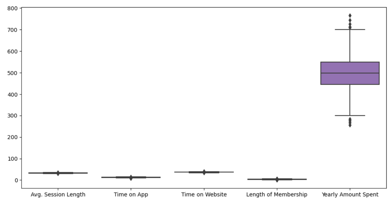
3) 특성들만 boxplot
plt.figure(figsize=(12,6))
sns.boxplot(data=data.iloc[:,:-1])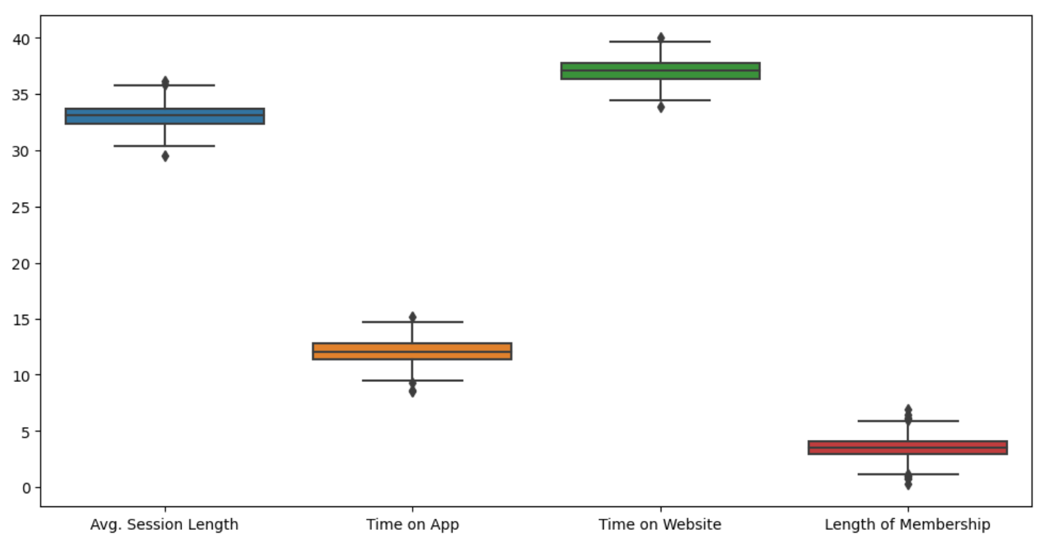
4) 라벨 값 boxplot
plt.figure(figsize=(12,6))
sns.boxplot(data=data['Yearly Amount Spent'])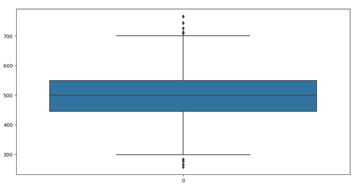
5) pairplot으로 경향 확인
plt.figure(figsize=(12,6))
sns.pairplot(data=data)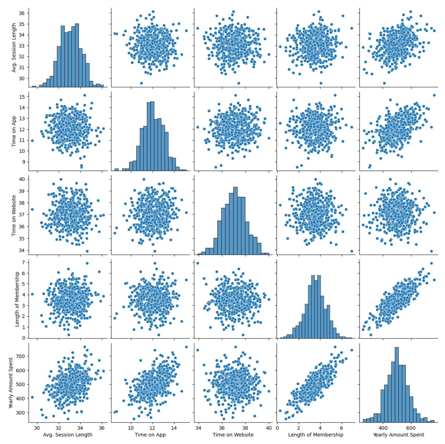
- 큰 상관관계를 보이는 것은 멤버쉽 유지 기간
3. 통계적 회귀
1) lmplot로 Yearly Amount Spent' , 'Length of Membership 확인
plt.figure(figsize=(12,6))
sns.lmplot(x='Yearly Amount Spent',y='Length of Membership',data=data)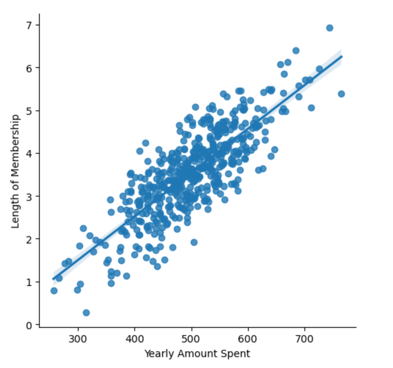
2) 상관이 높은 멤버쉽 유지기간만 가지고 통계적 회귀
import statsmodels.api as sm

X = data['Length of Membership']
y = data['Yearly Amount Spent']

lm = sm.OLS(y,X).fit()
lm.summary()

# 리포트
OLS Regression Results
Dep. Variable:	Yearly Amount Spent	R-squared (uncentered):	0.970
Model:	OLS	Adj. R-squared (uncentered):	0.970
Method:	Least Squares	F-statistic:	1.617e+04
Date:	Fri, 09 Dec 2022	Prob (F-statistic):	0.00
Time:	11:27:57	Log-Likelihood:	-2945.2
No. Observations:	500	AIC:	5892.
Df Residuals:	499	BIC:	5897.
Df Model:	1
Covariance Type:	nonrobust
coef	std err	t	P>|t|	[0.025	0.975]
Length of Membership	135.6117	1.067	127.145	0.000	133.516	137.707
Omnibus:	1.408	Durbin-Watson:	1.975
Prob(Omnibus):	0.494	Jarque-Bera (JB):	1.472
Skew:	0.125	Prob(JB):	0.479
Kurtosis:	2.909	Cond. No.	1.00
3) 좀 더 수치의 의미를 해석하려 해보자
- R-squared : 모형 적합도, y의 분산을 각각의 변수들이 약 99.8%로 설명할 수 있음
- Adj. R-squared : 독립변수가 여러 개인 다중회귀분석에서 사용
- Prob. F-Statistic : 회귀모형에 대한 통계적 유의미성 검정.(이 값이 0.05 이하라면 모집단애서도 의미가 있다고 볼수 있다)
(1) 회귀 모델을 그리기
pred = lm.predict(X)

sns.scatterplot(x=X, y=y)
plt.plot(X, pred, 'r', ls='dashed', lw=3)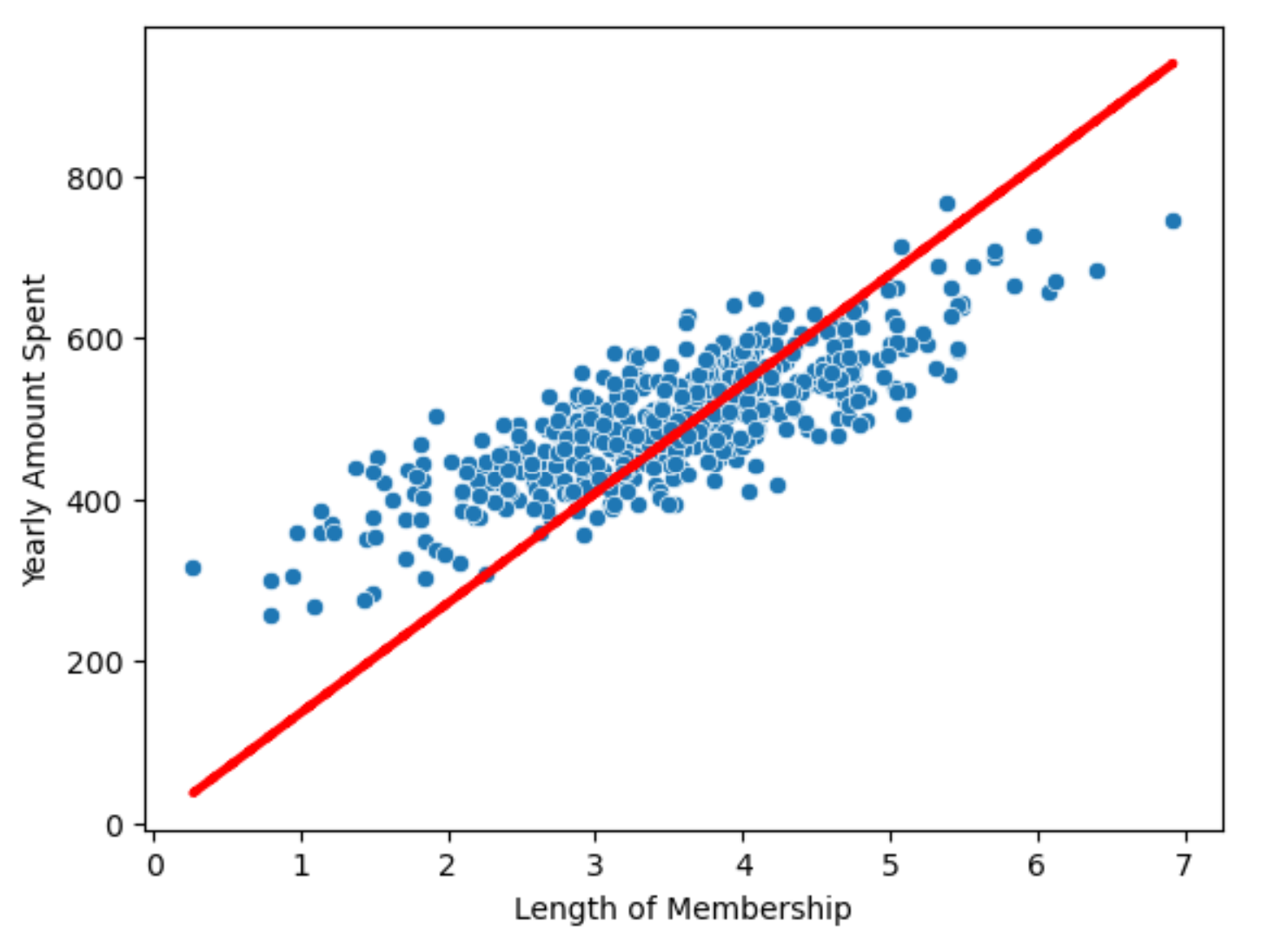
# 상수항이없어 직선에 문제가 있음 -> 상수항을 넣어주자
X = np.c_[X, [1]*len(X)]
X[:5]

# 선형회귀 결과
sns.scatterplot(x=X[:,0], y=y)
plt.plot(X[:,0], pred, 'r', ls='dashed', lw=3)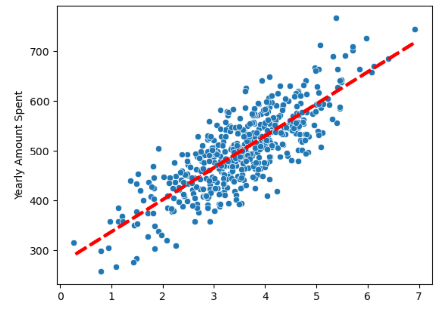
4) 데이터 분리
from sklearn.model_selection import train_test_split

X = data.drop('Yearly Amount Spent', axis= 1)
y = data['Yearly Amount Spent']

X_train, X_test , y_train, y_test = train_test_split(X, y, test_size=0.3, random_state=13)

# 4개의 컬럼 모두를 변수로 보고 회귀
import statsmodels.api as sm

lm = sm.OLS(y_train, X_train).fit()
lm.summary()

# 리포트
OLS Regression Results
Dep. Variable:	Yearly Amount Spent	R-squared (uncentered):	0.998
Model:	OLS	Adj. R-squared (uncentered):	0.998
Method:	Least Squares	F-statistic:	4.179e+04
Date:	Fri, 09 Dec 2022	Prob (F-statistic):	0.00
Time:	11:49:35	Log-Likelihood:	-1591.7
No. Observations:	350	AIC:	3191.
Df Residuals:	346	BIC:	3207.
Df Model:	4
Covariance Type:	nonrobust
coef	std err	t	P>|t|	[0.025	0.975]
Avg. Session Length	11.8431	0.906	13.070	0.000	10.061	13.625
Time on App	35.2169	1.212	29.046	0.000	32.832	37.602
Time on Website	-14.2536	0.840	-16.960	0.000	-15.907	-12.601
Length of Membership	60.1702	1.275	47.183	0.000	57.662	62.678
Omnibus:	0.648	Durbin-Watson:	2.013
Prob(Omnibus):	0.723	Jarque-Bera (JB):	0.755
Skew:	-0.042	Prob(JB):	0.686
Kurtosis:	2.788	Cond. No.	55.7
5) 참값 vs 예측값
sns.scatterplot(x=y_test, y=pred)
plt.plot([min(y_test), max(y_test)], [min(y_test), max(y_test)], 'r')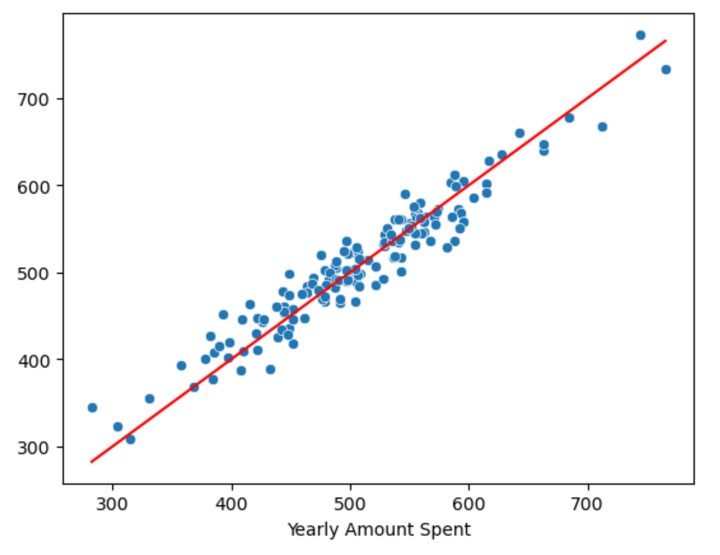

스터디 노트