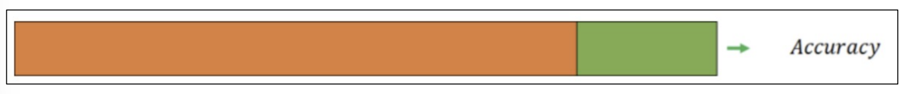
1. 교차검증
- 과적합 : 모델이 학습 데이터에만 과도하게 최적화된 현상.
그로 인해 일반화된 데이터에서는 예측 성능이 과하게 떨어지는 현상 - 주어진 데이터에 적용한 모델의 성능을 정확히 표현하기 위해서도 유용하다
1) holdout
2) k-fold cross validation
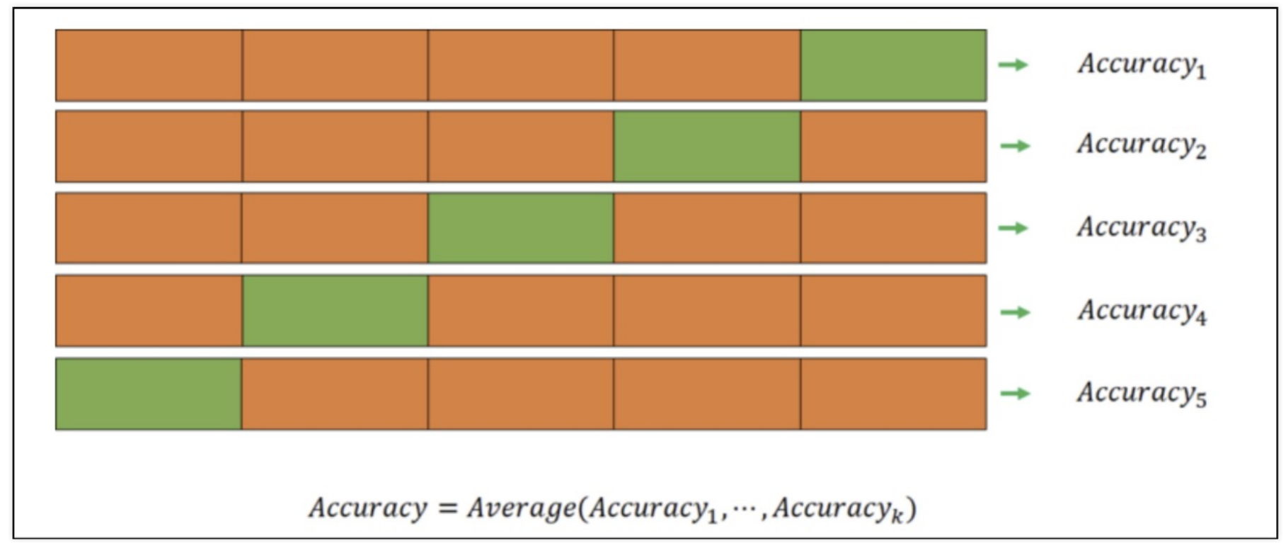
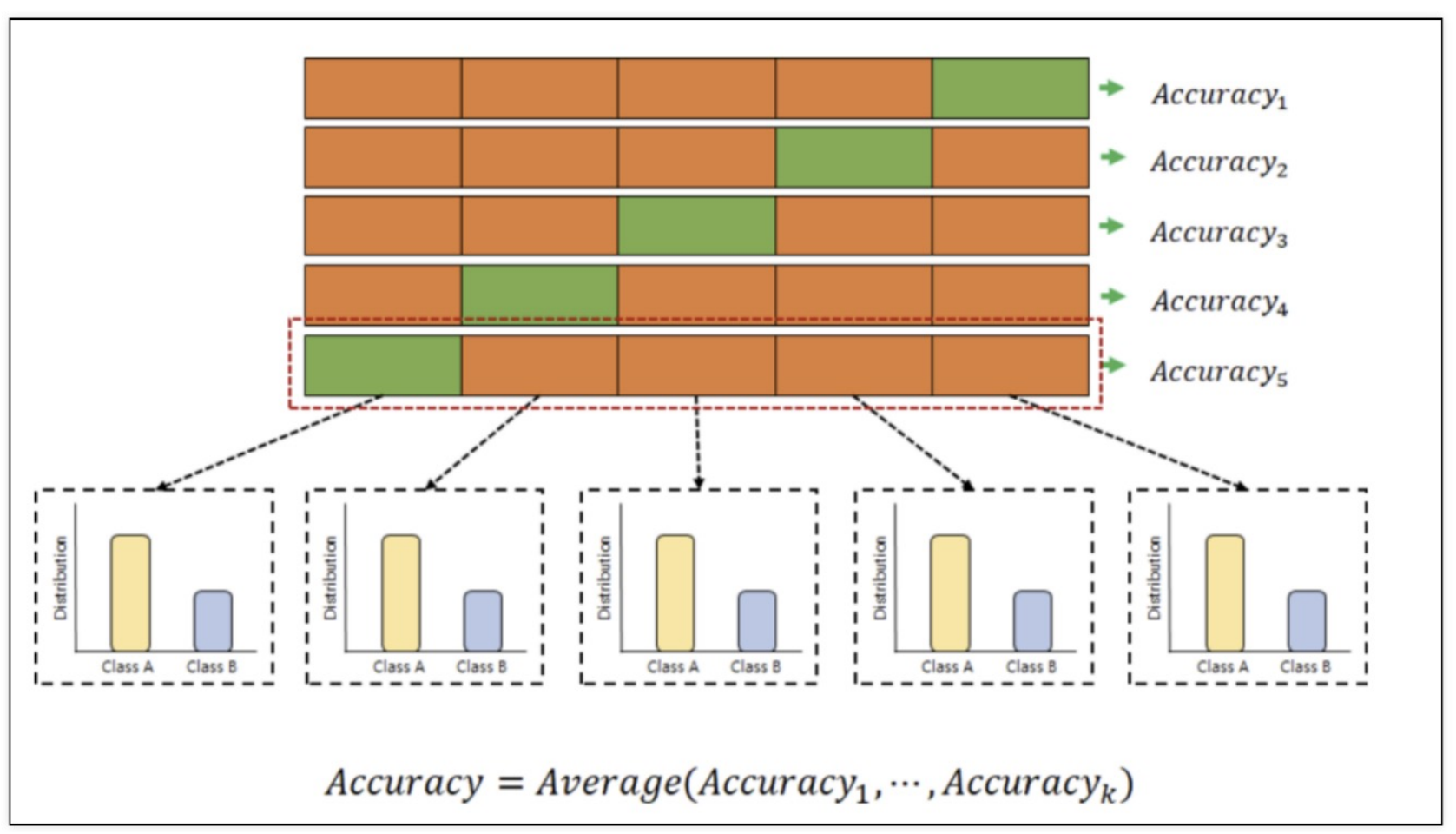
- 검증 validation이 끝난 후 test용 데이터로 최종 평가
3) 교차검증 간단하게 구현하기
import numpy as np
from sklearn.model_selection import KFold

X = np.array([
        [1,2], [3,4], [1,2], [3,4]
    ])
y = np.array(
        [1, 2, 3, 4]
    )

kf = KFold(n_splits = 2) # n_splits : 몇등분으로 할껀지(K-fold 에서 K번 하겠다)

print(kf.get_n_splits(X))
print(kf)

# 2
# KFold(n_splits=2, random_state=None, shuffle=False)
for train_idx, test_idx in kf.split(X):
    print('--- idx')
    print(train_idx, test_idx)
    print('--- train data')
    print(X[train_idx])
    print('--- val data')
    print(X[test_idx])

--- idx
[2 3] [0 1]
--- train data
[[1 2]
 [3 4]]
--- val data
[[1 2]
 [3 4]]
--- idx
[0 1] [2 3]
--- train data
[[1 2]
 [3 4]]
--- val data
[[1 2]
 [3 4]]
2. K-fold, Stratified K-Fold 와인 분류기
1) 와인데이터 가져오기
import pandas as pd

red_url = 'https://raw.githubusercontent.com/PinkWink/ML_tutorial/master/dataset/winequality-red.csv'
white_url = 'https://raw.githubusercontent.com/PinkWink/ML_tutorial/master/dataset/winequality-white.csv'

red_wine = pd.read_csv(red_url, sep= ';')
white_wine = pd.read_csv(white_url, sep= ';')

red_wine['color'] = 1.
white_wine['color'] = 0.

wine = pd.concat([red_wine, white_wine])

# 와인 맛 분류기를 위한 데이터 정리
wine['taste'] = [1. if grade > 5 else 0. for grade in wine['quality']]

X = wine.drop(['taste', 'quality'], axis = 1)
y = wine['taste']
2) K-Fold
(1) KFold
from sklearn.model_selection import KFold

kfold = KFold(n_splits=5)
wine_tree_cv = DecisionTreeClassifier(max_depth=2, random_state=13)
(2) KFold는 index를 반환한다
# 길이 확인해보기
for train_idx, test_idx in kfold.split(X):
    print(len(train_idx),len(test_idx))

5197 1300
5197 1300
5198 1299
5198 1299
5198 1299
(3) 각각의 fold에 대한 학습 후 acc
cv_accuracy = [] # 검증마다 성능 기록 보관

for train_idx, test_idx in kfold.split(X):
    X_train = X.iloc[train_idx]
    X_test = X.iloc[test_idx]
    y_train = y.iloc[train_idx]
    y_test = y.iloc[test_idx]

    wine_tree_cv.fit(X_train, y_train)
    pred = wine_tree_cv.predict(X_test)
    cv_accuracy.append(accuracy_score(y_test, pred))

# cv_accuracy
[0.6007692307692307,
 0.6884615384615385,
 0.7090069284064665,
 0.7628945342571208,
 0.7867590454195535]
# 분산이 크지 않다면 평균값을 대표 값으로 한다
np.mean(cv_accuracy)

# 0.709578255462782
3) Stratified K-Fold 사용
(1) StratifiedKFold 학습 후 Acc
from sklearn.model_selection  import StratifiedKFold

skfold = StratifiedKFold(n_splits=5)
wine_tree_cv = DecisionTreeClassifier(max_depth=2, random_state=13)

cv_accuracy = []

for train_idx, test_idx in skfold.split(X, y):
    X_train = X.iloc[train_idx]
    X_test = X.iloc[test_idx]
    y_train = y.iloc[train_idx]
    y_test = y.iloc[test_idx]

    wine_tree_cv.fit(X_train, y_train)
    pred = wine_tree_cv.predict(X_test)
    cv_accuracy.append(accuracy_score(y_test, pred))

# cv_accuracy
[0.5523076923076923,
 0.6884615384615385,
 0.7143956889915319,
 0.7321016166281755,
 0.7567359507313318]
4) cross validation을 보다 간편하게 사용
from sklearn.model_selection import cross_val_score

skfold = StratifiedKFold(n_splits=5)
wine_tree_cv = DecisionTreeClassifier(max_depth=2, random_state=13)

cross_val_score(wine_tree_cv, X, y, scoring=None, cv= skfold)

# array([0.55230769, 0.68846154, 0.71439569, 0.73210162, 0.75673595])
from sklearn.model_selection import cross_val_score
skfold = StratifiedKFold(n_splits=5)
wine_tree_cv = DecisionTreeClassifier(max_depth=5, random_state=13)
cross_val_score(wine_tree_cv, X, y, scoring=None, cv= skfold)
# array([0.50076923, 0.62615385, 0.69745958, 0.7582756 , 0.74903772])- depth가 높다고 무조건 acc가 좋아지는 것이 아니다
5) skfold를 함수로 만들어보자
def skfold(depth):
    from sklearn.model_selection import cross_val_score

    skfold = StratifiedKFold(n_splits=5)
    wine_tree_cv = DecisionTreeClassifier(max_depth=depth, random_state=13)

    print(cross_val_score(wine_tree_cv, X, y, scoring=None, cv= skfold))
3. 하이퍼파라미터 튜닝
- 모델의 성능을 확보하기 위해 조절하는 설정 값
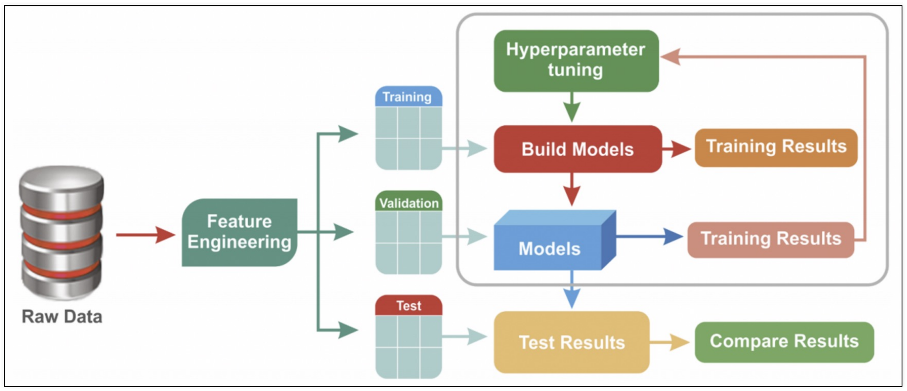
- 튜닝 대상
- 결정나무에서 아직 우리가 튜닝해 볼만한 것은 max_depth이다.
- 간단하게 반복문으로 max_depth를 바꿔가며 테스트해볼 수 있을 것이다.
- 그런데 앞으로를 생각해서 보다 간편하고 유용한 방법을 생각해보자
1) 와인데이터 하이퍼파라미터 적용
import pandas as pd

red_url = 'https://raw.githubusercontent.com/PinkWink/ML_tutorial/master/dataset/winequality-red.csv'
white_url = 'https://raw.githubusercontent.com/PinkWink/ML_tutorial/master/dataset/winequality-white.csv'

red_wine = pd.read_csv(red_url, sep= ';')
white_wine = pd.read_csv(white_url, sep= ';')

red_wine['color'] = 1.
white_wine['color'] = 0.

wine = pd.concat([red_wine, white_wine])

wine['taste'] = [1. if grade > 5 else 0. for grade in wine['quality']]

X = wine.drop(['taste', 'quality'], axis = 1)
y = wine['taste']
2) GridSearchCV
- 결과를 확인하고 싶은 파라미터를 정의
- cv는 cross validation
from sklearn.model_selection import GridSearchCV
from sklearn.tree import DecisionTreeClassifier

params = {'max_depth' : [2, 4, 7, 10]}
wine_tree = DecisionTreeClassifier(max_depth=2, random_state=13)

gridsearch = GridSearchCV(estimator=wine_tree, param_grid=params, cv=5)
gridsearch.fit(X, y)
{ 'mean_fit_time': array([0.00618343, 0.00903974, 0.01902323, 0.02739959]),
'mean_score_time': array([0.00142026, 0.00100141, 0.0021904 , 0.00161719]),
'mean_test_score': array([0.6888005 , 0.66356523, 0.65340854, 0.64401587]),
'param_max_depth': masked_array(data=[2, 4, 7, 10],
mask=[False, False, False, False],
fill_value='?',
dtype=object),
'params': [ {'max_depth': 2},
{'max_depth': 4},
{'max_depth': 7},
{'max_depth': 10}],
'rank_test_score': array([1, 2, 3, 4]),
'split0_test_score': array([0.55230769, 0.51230769, 0.50846154, 0.51615385]),
'split1_test_score': array([0.68846154, 0.63153846, 0.60307692, 0.60076923]),
'split2_test_score': array([0.71439569, 0.72363356, 0.68360277, 0.66743649]),
'split3_test_score': array([0.73210162, 0.73210162, 0.73672055, 0.71054657]),
'split4_test_score': array([0.75673595, 0.7182448 , 0.73518091, 0.72517321]),
'std_fit_time': array([1.27047707e-03, 8.17307235e-05, 2.82734019e-03, 5.54786581e-03]),
'std_score_time': array([8.39471892e-04, 1.81824455e-06, 1.16665998e-03, 5.03435946e-04]),
'std_test_score': array([0.07179934, 0.08390453, 0.08727223, 0.07717557])}- n_jobs 옵션을 높여주면 CPU의 코어를 보다 병렬로 활용함. Core가 많으면 n_jobs를 높이면 속도가 빨라진다
3) GridSearchCV의 결과
import pprint

pp = pprint.PrettyPrinter(indent=4)
pp.pprint(gridsearch.cv_results_)
{ 'mean_fit_time': array([0.00618343, 0.00903974, 0.01902323, 0.02739959]),
'mean_score_time': array([0.00142026, 0.00100141, 0.0021904 , 0.00161719]),
'mean_test_score': array([0.6888005 , 0.66356523, 0.65340854, 0.64401587]),
'param_max_depth': masked_array(data=[2, 4, 7, 10],
mask=[False, False, False, False],
fill_value='?',
dtype=object),
'params': [ {'max_depth': 2},
{'max_depth': 4},
{'max_depth': 7},
{'max_depth': 10}],
'rank_test_score': array([1, 2, 3, 4]),
'split0_test_score': array([0.55230769, 0.51230769, 0.50846154, 0.51615385]),
'split1_test_score': array([0.68846154, 0.63153846, 0.60307692, 0.60076923]),
'split2_test_score': array([0.71439569, 0.72363356, 0.68360277, 0.66743649]),
'split3_test_score': array([0.73210162, 0.73210162, 0.73672055, 0.71054657]),
'split4_test_score': array([0.75673595, 0.7182448 , 0.73518091, 0.72517321]),
'std_fit_time': array([1.27047707e-03, 8.17307235e-05, 2.82734019e-03, 5.54786581e-03]),
'std_score_time': array([8.39471892e-04, 1.81824455e-06, 1.16665998e-03, 5.03435946e-04]),
'std_test_score': array([0.07179934, 0.08390453, 0.08727223, 0.07717557])}# 최적의 성능을 가진 모델
gridsearch.best_estimator_,
# (DecisionTreeClassifier(max_depth=2, random_state=13)
gridsearch.best_params_,
# {'max_depth': 2}
gridsearch.best_score_
# 0.6888004974240539)4. Pipeline을 적용한 모델에 GridSearch를 적용하기
1) Pipeline
from sklearn.pipeline import Pipeline
from sklearn.tree import DecisionTreeClassifier
from sklearn.preprocessing import StandardScaler

estimators = [
        ('scaler', StandardScaler()),
        ('clf', DecisionTreeClassifier(random_state=13))
    ]

pipe = Pipeline(estimators)
2) GridSearch
param_grid = [{'clf__max_depth' : [2,4,7,10]}]

Gridsearch = GridSearchCV(estimator = pipe, param_grid = param_grid, cv= 5)
Gridsearch.fit(X,y)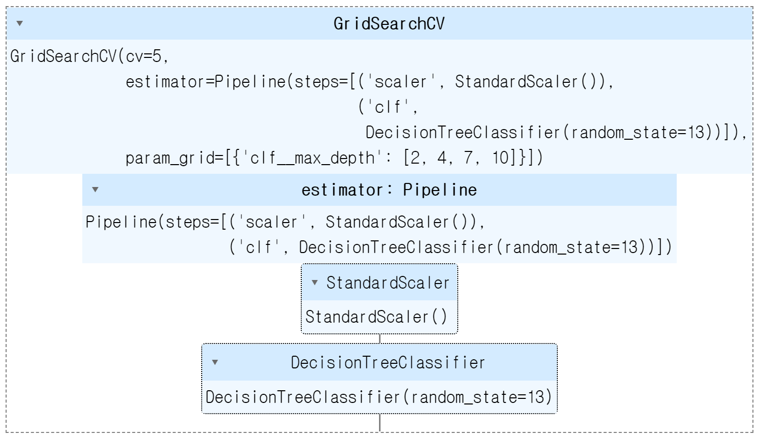
Gridsearch.best_estimator_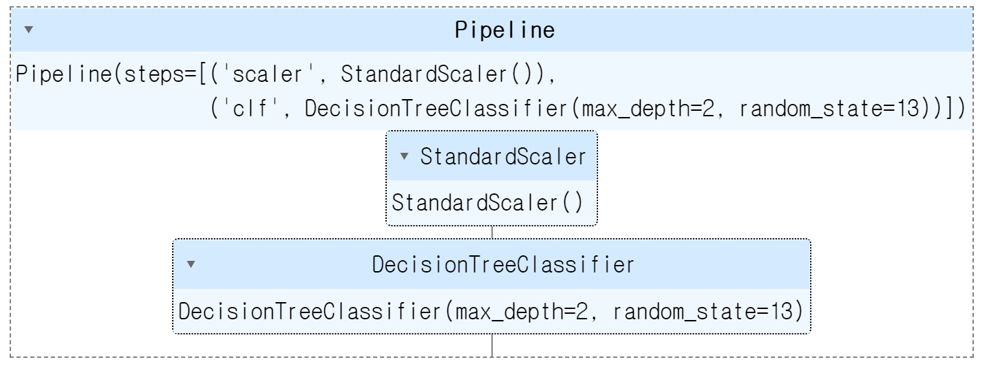
Gridsearch.best_score_
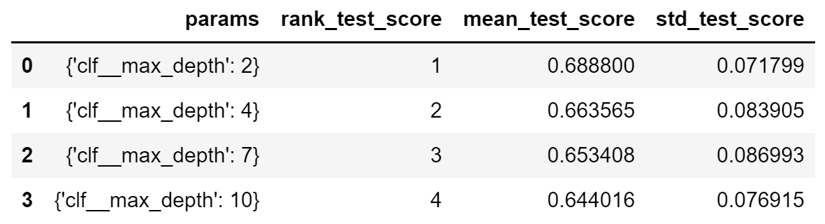
# 0.68880049742405393) 표로 성능 결과 정리
import pandas as pd

score_df = pd.DataFrame(Gridsearch.cv_results_)
score_df[
	['params', 'rank_test_score', 'mean_test_score', 'std_test_score']
    ]

스터디 노트