Computer vision 개념들을 해당 포스트에 지속적으로 업데이트하며 정리하겠습니다! 필요한 개념이 있으시다면, 검색하면서 찾아보시는 것이 좋을 것 같아요!
2D Points
2D points in inhomogeneous coordinates
x=(xy)∈R2
2D points in homogeneous coordinates
x~=⎝⎜⎛x~y~w~⎠⎟⎞∈R2
- homogeneous 좌표계에선 scale만 다른 벡터는 동일한 벡터임! ex) (2, 2, 2) = (1, 1, 1)
2D points in homogeneous coordinates ↔ inhomogeneous coordinates
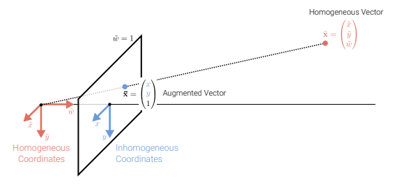
xˉ=(x1)=x~=⎝⎜⎛xy1⎠⎟⎞=w~1x~=w~1⎝⎜⎛x~y~w~⎠⎟⎞=⎝⎜⎛x~/w~y~/w~1⎠⎟⎞
2D lines
{xˉ∣l~Txˉ=0}⟺{x,y∣ax+by+c=0}
- l~=(a,b,c)T
- normalize! → l~=(nx,ny,d)T=(n,d)T, ∣∣n∣∣2=1
2D Line Arithmetic
- intersection of two lines: x~=l~1×l~2
- line joining two points: l~=xˉ1×xˉ2
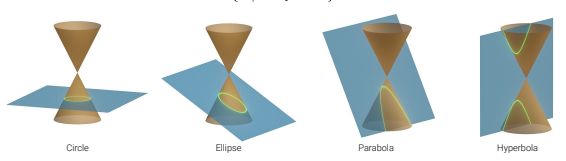
2D conics
평면과 3D 콘의 교차평면!
multi-view geometry, camera calibraion에 유용!
{xˉ∣xˉTQxˉ=0}
3D Points
3D points in inhomogeneous coordinates
x=⎝⎜⎛xyz⎠⎟⎞∈R3
3D points in homogeneous coordinates
x~=⎝⎜⎜⎜⎛x~y~w~z~⎠⎟⎟⎟⎞∈R3
3D plains
{xˉ∣m~Txˉ=0}⟺{x,y,z∣ax+by+cz+d=0}
- m~=(a,b,c)T
- normalize! → l~=(nx,ny,nz,d)T=(n,d)T, ∣∣n∣∣2=1
3D lines
{x∣(1−λ)p+λq∧λ∈R}
- 선에 놓인 two points p,q의 선형 결합으로 표현 가능.
- two-plane parameterization으로 표현하는 것도 가능.
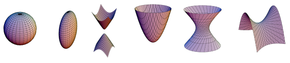
3D Qudadrics
2D conics의 3D 아날로그가 quadric surface임. multi-view geometry에서 사용
{xˉ∣xˉTQxˉ=0}
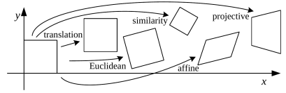
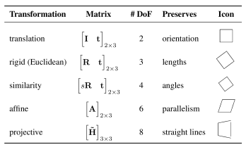
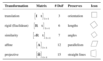
Translation
- 좌표 이동 / 2 DoF(Degrees of Freedom)
- homogeneous(투영) 좌표계를 사용하여 chain, invert transformation 가능!
x′=x+t⟺xˉ′=[I0Tt1]xˉ
Euclidean
- 좌표 이동 + 회전 / 3 DoF(Degrees of Freedom)
- R∈SO(2): 직교 회전 행렬! (RRT=I, det(R)=1)
- 유클리디언 변환은 유클리디언 거리를 보존함!
x′=x+Rx⟺xˉ′=[R0Tt1]xˉ
Similarity
- 좌표 이동 + 회전 with scale / 4 DoF(Degrees of Freedom)
- 두 선 사이의 각도 보존!
x′=x+sRx⟺xˉ′=[sR0Tt1]xˉ
Affine
- 모든 2차원 선형 변환! / 6 DoF(Degrees of Freedom)
- A∈R2×2: 임의의 2 x 2 행렬
- 평행한 선은 평행하게 보존!
x′=x+Ax⟺xˉ′=[A0Tt1]xˉ
Projective
- Homography! / 8 DoF(Degrees of Freedom)
- H∈R3×3: 임의의 homogeneous 행렬
- 일직선(straight)은 일직선으로 보존!
- 전치 역행렬을 통해서 co-vector의 Projective 변환을 나타내는 것도 가능함!
- l~′=H~−Tl~
x~′=H~x~
(2D 변환과 유사하기 때문에 생략!)
두 homogeneous 벡터에 대해서 Homograpy를 추정하는 방법.
- X={x~i,x~i′}i=1N: a set of N개의 2D-to-2D correspondences by x~i′=H~x~iT (Homography)
- 이때 두 벡터는 방향이 같으므로, x~i′×H~x~i=0의 방정식을 가짐. → 아래의 식으로 표현 가능!
⎣⎢⎡0Tw~i′x~i′T−y~i′x~i′T−w~i′x~i′T0Tx~i′x~i′Ty~i′x~i′T−x~i′x~i′T0T⎦⎥⎤⎣⎢⎡h~1h~2h~3⎦⎥⎤=0
- Ai=⎣⎢⎡0Tw~i′x~i′T−y~i′x~i′T−w~i′x~i′T0Tx~i′x~i′Ty~i′x~i′T−x~i′x~i′T0T⎦⎥⎤
- h~=⎣⎢⎡h~1h~2h~3⎦⎥⎤/ h~kT: Homography 행렬의 k번째 행!
A행렬을 2N x 9 행렬로 쌓은 후, least square 문제를 해결하는 것으로 Homography를 추정할 수 있음!! + 위 방정식의 optimal solution은 SVD의 가장 작은 특이값에 해당하는 고유벡터와 같다! 궁금하다면, 블로그 내용 참고 특이값 분해(SVD) - gaussian37
h~∗=h~argmin∣∣Ah~∣∣22+λ(∣∣h~∣∣22−1)=h~argminh~TA~TAh~+λ(h~Th~−1)
Projection Models
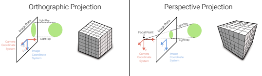
Orthographic Projection
- Focal length가 길 경우에 사용(천체 관측)
- 각 ray가 카메라 좌표계(z축)와 평행함
Perspective Projection
- 카메라 센터, focal point로 빛이 통과
- Object size 바뀜
Orthographic Projection
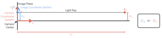
orthographic projection은 좌표의 z 성분을 드랍하는 것으로 적용됨.
xs=[100100]xc⟺xˉs=⎣⎢⎡100010000001⎦⎥⎤xˉc
- scale 적용하는 것도 가능. s: px/m or px/mm (for 3D points → pixels)
Perspective Projection
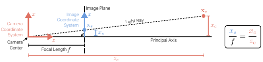
perspective projection은 z 성분을 나누는 것으로 사영하는 방법임.
(xsys)=(fxc/zcfyc/zc)⟺x~s=⎣⎢⎡f000f0001000⎦⎥⎤xˉc
Principal Point Offset
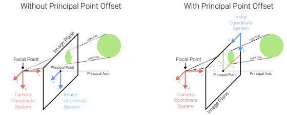
- pixel 좌표계를 positive(0~255)로 유지하기 위하여, offset c 설정! → image plane의 코너로 좌표계 옮김
(xsys)=(fxc/zc+syc/zc+cxfyc/zc+cy)⟺x~s=⎣⎢⎡fx00sfy0cxcy1000⎦⎥⎤xˉc
- K=⎣⎢⎡fs00sfy0cxcy1⎦⎥⎤:
calibration matrix K , K의 파라미터 = camera intrinsics
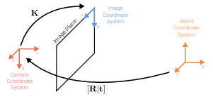
- K: calibration matrix(intrinsics)
- [R∣t]: camera pose(extrinsics)
x~s=[K0]xˉc=[K0][R0Tt1]xˉw=Pxˉw
- xˉs=x~s/zs=(xs/zs,ys/zs,1,1/zs)T → 4번째 값: inverse depth
- inverse depth 알고 있으면 pixel 좌표로부터 3D point 얻을 수 있음!
Lens Distortion
카메라 렌즈의 왜곡 현상 때문에, linear projection의 추정이 달라지게 됨.
x′=(1+κ1γ2+κ2γ4)(xy)+(2κ3xy+κ4(γ2+2x2)2κ4xy+κ3(γ2+2y2))=(x′y′)
xs=(fxx′+cxfyy′+cy)
- Radial Distortion: (1+κ1γ2+κ2γ4)
- Tangential Distortion: (2κ3xy+κ4(γ2+2x2)2κ4xy+κ3(γ2+2y2))
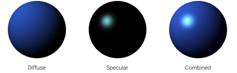
위에서는 픽셀과 컬러에 대해서 이미지를 살펴보았다면, 지금부턴 반사 or 굴절 등에 의해 빛이 방출되어 발생하는 효과들에 대한 개념임.
Rendering Equation
Lout(p,v,λ)=Lemit(p,v,λ)+∫ΩBRDF(p,s,v,λ)⋅Lin(p,s,λ)⋅(−nTs)ds
- Ω: 단위 반구 at normal n
- BDRF: Bidirectional Reflectance Distribution Function → 빛이 불투명한 표면에서 어떻게 반사되는지 정의
- (−nTr) - attenuation equation (if light arrives exactly perpendicular, there is no reflectance at all. or if it arrives at a shallow angle, there is less light reflected).
- Lemit>0: 표면이 빛을 방출할 때만!
Fresnel Effect
- 바라보는 각도에 따라 표면으로부터 빛이 반사되는 양
Global Illumination
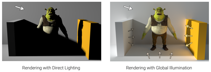
- Occulusion 등의 현상으로 하나의 빛으로는 렌더링이 불충분할 때 사용
Camera Lenses
- 렌즈 없이 핀홀만을 사용하게 되면, 이미지에 blur 효과가 발생함! (핀홀 크기 클 경우 → averaging, 핀홀 크기 작을 경우 → diffraction + shutter time 매우 길어져 motion blur 유발)
- 따라서 렌즈로 충분한 양의 빛을 얻어 이미지를 얻어냄!
- 하지만 focus, vignetting, aberration은 조정해야 함
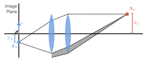
Thin Lens Model
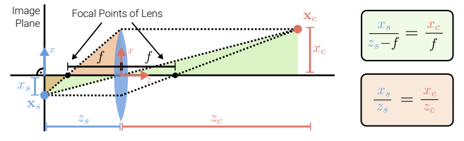
- 초록색 박스: 빨간색 삼각형 비율
- 빨간색 박스: 초록색 삼각형 비율
- f: focal length of the lens.
xcxs→fzs−f=zczs→zs1+zc1=f1
- thin lens model은 approximation에 주로 사용함.
- z축과 평행한 rays가 focal point 통과함
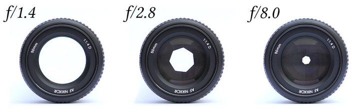
Depth of Field
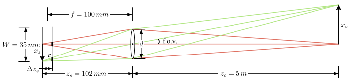
- zs1+zc1=f1를 만족할 때 이미지가 in focus(초점)인 상태임.
- out of focus일 때, 3D points가 circle of confusion c로 사영됨.
- 이 c를 제한하는 depth variation이 depth of field이며, focus distance와 lens aperture의 함수로도 볼 수 있음. → lens aperture(노출도)를 조절하여 c의 사이즈를 조정!
N=df(often denoted as f/N)
Chromatic Aberration
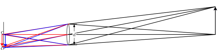
- 다른 색들에 대해 빛이 약간 다른 거리에서 초점이 맞춰지는 경향을 의미함.
- 해결방법: 다양한 유리 재질로 렌즈 구성하기.
Vignetting
- 이미지 edge에서 밝기가 떨어지는 현상임.
- 자연적 요인: 피사체의 표면을 무한하게 볼 수 없음 + 렌즈 노출도
- 기계적 요인: 광선의 그늘진 부분(그림 참고)이 이미지에 도달 불가능
- calibration으로 해결 가능.
Image Sensing Pipeline
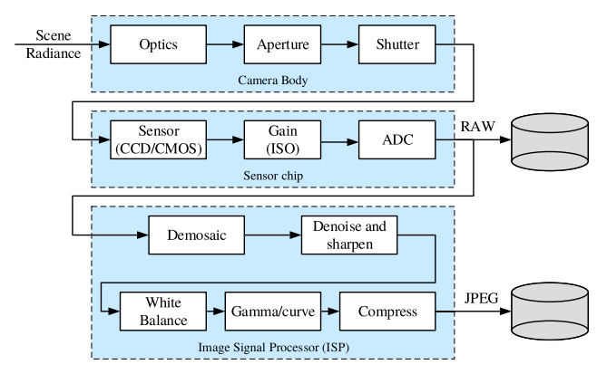
Image sensing pipeline은 다음 세 가지 단계로 구성됨.
- Physical light transport (in the camera body)
- Photon measurement (on the sensor chip)
- Image signal processing
Shutter
- 셔터 스피드 → 빛이 센서에 얼마나 들어올지 조정
- 셔터를 통해 이미지의 밝기, 흐림, 노이즈 정도가 결정됨.
Sensor
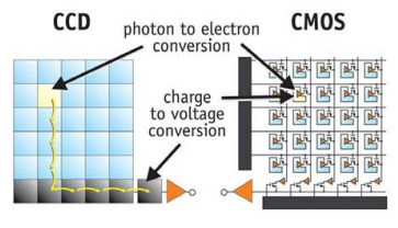
Color Filter Arrays
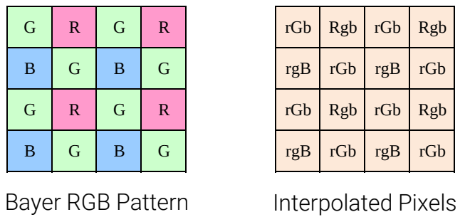
- 이미지의 color 값 얻기 위해 사용! (센서만으로는 불가능.)
Gamma Compression
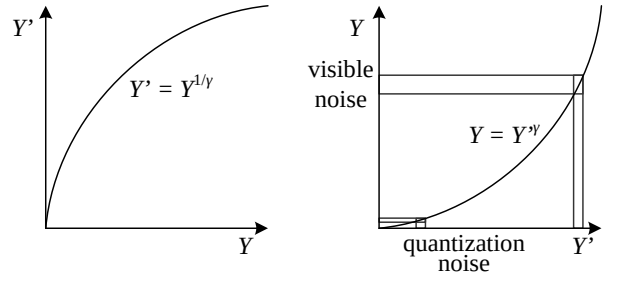
- 인간은 어두운 환경에서 눈이 민감하게 반응함 → 비선형적으로 강도나 색을 변형해야 함.
Image Compression
- 우리가 흔히 아는 이미지 압축
- 8 x 8 patch-based discrete cosine or wavelet transforms 사용!
- Discrete Cosine Transform: 자연 이미지에 PCA 적용하는 것과 유사
Reference
[1] Andreas Geiger, Computer vision (2023)