High-Resolution Image Synthesis with Latent Diffusion Models

김민솔·2024년 4월 4일

Diffusion

목록 보기

4/5

길었던 diffusion models 시리즈에 중요한 챕터인 Latent Diffusion Model(Stable Diffusion)까지 오게 되었습니다.. LDM이 가져온 파장이 현재 인공지능 분야 중 생성 모델이 가장 뜨거운 분야가 되게 만들었다고 봐도 무방할 것 같네요. LDM은 앞에서 봤던 DDPM과 Score-based models, DDIM과 같은 선행 지식들을 Latent space에 적용한 모델입니다. 이제부터 LDM에 대해서 자세히 살펴보겠습니다.

Introduction

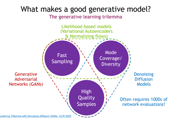
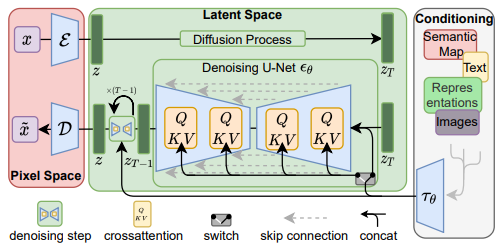
Denoising Diffusion models은 Mode Coverage/Diversity나 High Quality Samples의 측면에서는 뛰어난 성능을 보였습니다. 하지만 샘플링 속도가 GAN 계열 모델에 비해, 현저하게 느리다는 것이 단점입니다. 이를 해결하기 위해 score-based models, DDIM, Distillation 등의 방법들이 사용되었던 것입니다. LDM에서는 제한된 연산 내에서 Sample의 퀄리티와 다양성을 보존하기 위하여 latent space에서 diffusion 과정을 적용시켰습니다. Pretrained AutoEncoder를 사용하여 input images를 Pixel space에서 Latent space로 매핑합니다. 이후 우리가 아는 Diffusion process와 Reverse process를 적용하고, Pretrained AE로 이미지를 복원합니다. LDM이 가지는 주요 특징들은 다음과 같습니다.

고차원의 데이터를 압축시켜 사용하기 때문에, 고해상도의 이미지들에 적용될 수 있습니다. + inpainting이나 super-resolution과 같은 conditioned tasks에는 $1024^2$ 픽셀까지 생성이 가능합니다.
다양한 tasks에 적용 가능합니다. (e.g. image synthesis, inpainting, …)
cross-attention 메커니즘을 사용하여 multi-modal이 가능합니다. (e.g. text-to-image)
AutoEncoder는 pretrained model로 사용합니다.

Methods

Latent space에서 diffusion 모델을 적용하는 것이 어떤 의미를 가질까요? image space가 아닌 latent space에서 generative modeling을 실행하게 되면, low-dimensional space에서 high-dimensional data를 생성하는 것이 가능합니다. 따라서 연산도 효율적이고, 퀄리티도 유지할 수 있습니다. 지금부터는 LDM에 사용된 methods에 대해서 하나씩 살펴보겠습니다.

1. Perceptual Image Compression

Perceptual Compression model은 이전 연구와 같이 perceptual loss와 patch-based adversarial objective의 결합으로 학습된 Autoencoder에 기초하여 구성되었습니다. 이를 통해 image blur 현상을 피하고, local적인 부분들도 좋은 성능으로 생성합니다.

이미지 $x \in \Reals^{H \times W \times 3}$ 가 주어지면, encoder $\mathcal{E}$ 가 $x$ 를 latent space로 매핑합니다. $z = \mathcal{E}(x)$ 그리고, decoder $\mathcal{D}$ 가 latent vector $z \in \Reals^{h \times w \times c }$ 로부터 이미지를 reconstruction합니다. $\tilde x = \mathcal{D}(z) = \mathcal{D}(\mathcal{E}(x))$ . 이때 encoder $\mathcal{E}$ 가 이미지를 매핑할 시 factor $f = H/h = W/w = 2^m$ 으로 downsampling합니다.

avoid high-variance latent spaces

High-variance space가 되는 것을 피하기 위하여 두 가지의 Regularization 방법을 사용하였습니다.

(1) KL-reg.

encode된 standard normal에 KL-penalty를 부여하는 방식입니다.

(2) VQ-reg.

decoder 내에 vector quantization layer를 사용하는 방식입니다. (:= VQGAN)

해당 reg term들을 통해 이전 연구보다 $x$ 의 디테일들을 더 보존할 수 있었습니다.

2. Latent Diffusion Models

Diffusion Models는 noised 정규 분포를 반복적으로 denoising하여 data dist. $p(x)$ 를 학습하는 확률 모델입니다. Diffusion models의 시초 격인 DDPM에서는 Denoising reverse process을 고정된 Markov Chain process로 설계하였습니다. 또한 Image synthesis에서 denoising score-matching과 같은 방법들을 사용합니다.

Diffusion models의 목적 함수는 다음과 같습니다.

L_{DM} = \mathbb{E}_{t \sim \mathcal{U}(1,T), x, \epsilon \sim \mathcal{N}(0,1)}\Big[||\epsilon-\epsilon_\theta(x_t, t)||^2_2\Big]

Latent representations로 generative modeling을 할 경우 연산이 더 효율적이고, high-frequency를 가지며, detail들을 축약하는 것이 가능합니다. 따라서 저차원의 space를 사용하게 되면, likelihood-based 생성 모델에 더 효율적입니다.

perceptual compression model(Pretrained AE)를 사용한 목적 함수는 다음과 같습니다.

L_{LDM} := \mathbb{E}_{t \sim \mathcal{U}(1,T), z=\mathcal{E}(x), \epsilon \sim \mathcal{N}(0,1)}\Big[||\epsilon-\epsilon_\theta(z_t, t)||^2_2\Big]

$\epsilon_\theta(\cdot, t)$ : time-conditional Unet
forward process 고정 → $\mathcal{E}$ 로부터 $z_t$ 얻기
$p(z)$ 로 얻어진 샘플은 $\mathcal{D}$ 를 통해 image space로 보냄.

3. Conditioning Mechanisms

Diffusion models는 이론적으로 conditional dist. $p(z|y)$ 를 모델링하는 것이 가능합니다. 따라서 denoising autoencoder에 condition을 추가하였습니다.

$\epsilon_\theta(z_t, t, y)$ : conditional denoising autoencoder
$y$ : inputs! (e.g. text, semantic maps, …)

Diffusion 모델이 다양한 input modality들을 통해 conditional image generation을 수행할 수 있도록, Unet 구조에 cross-attention을 적용하였습니다. 또한 $y$ 를 전처리하기 위하여 condition encoder $\tau_\theta(y) \in \Reals^{M \times d_\tau}$ 를 사용하였습니다.

\mathrm{Attention}(Q, K, V) = \mathrm{softmax}\big(\frac {QK^T} {\sqrt d} \big) \cdot V

$Q = W^{(i)}_Q \cdot \psi_i(z_t)$
- $W^{(i)}_Q \in \Reals^{d \times d^i_\epsilon}$
- $\psi_i(z_t) \in \Reals^{N \times d^i_\epsilon}$ : (flattened) Unet representation $\epsilon_\theta$
$K = W^{(i)}_K \cdot \tau_\theta(y)$
- $W^{(i)}_K \in \Reals^{d \times d_\tau}$
$V = W^{(i)}_V \cdot \tau_\theta(y)$
- $W^{(i)}_V \in \Reals^{d \times d_\tau}$

condition까지 고려한 LDM의 Loss는 다음과 같습니다.

L_{LDM} := \mathbb{E}_{t \sim \mathcal{U}(1,T), \mathcal{E}(x), \epsilon \sim \mathcal{N}(0,1)}\Big[||\epsilon-\epsilon_\theta(z_t, t,\tau_\theta(y))||^2_2\Big]

$\epsilon_\theta,\tau_\theta(y)$ 는 같이 최적화됨!

Experiments

LDM이 pixel-based DM에 비해 가지는 이점들을 파악하는 챕터입니다.

1. On Perceptual Compression Tradeoffs

해당 파트에서는 LDM의 downsampling factor $f \in \{1,2,4,8,16,32\}$ 에 따른 성능 변화를 살펴보았습니다. $f$ 가 작을 경우 training process가 느리다는 단점이 존재하며, $f$ 가 클 경우 이미지 fidelity 학습이 어렵다는 단점이 존재합니다. 따라서 LDM-{4-8}이 효율성과 샘플 퀄리티 면에서 가장 적당한 모델로 설정하였습니다.

2. Image Generation with Latent Diffusion

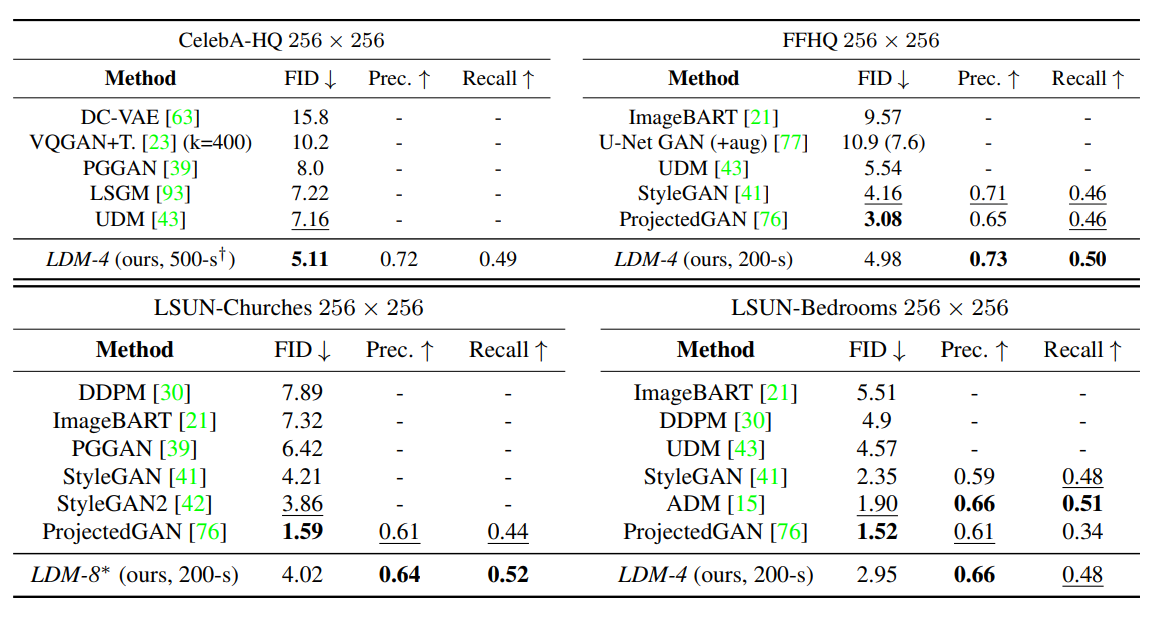
unconditional model을 $256^2$ 사이즈의 이미지셋에 평가한 표입니다. sample quality는 FID로, data manifold coverage는 Precision, Recall로 평가하였습니다.

CelebA-HQ 데이터셋에 대해서는 FID로 SOTA를 달성하였습니다. 또한 GAN-based 모델보다 mode-covering 성능이 모든 데이터셋에서 높은 점도 주목할 만합니다.

3. Conditional Latent Diffusion

cross-attention을 도입하여 다양한 modality를 모델에 적용 가능하도록 설계하였습니다. text-to-image task에서는 BERT-tokenizer와 $\tau_\theta$ 를 transformer로 구현하였습니다. 또한 classifier-free guidance를 적용하여 샘플 퀄리티를 향상시켰습니다.

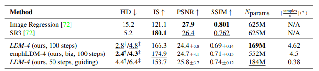
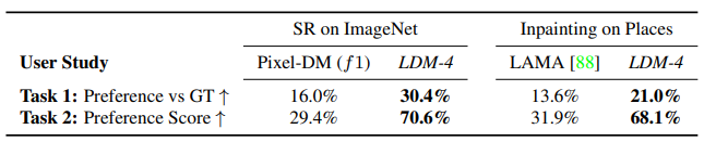
4. Super-resolution / Inpainting

$\epsilon_\theta$ 에 conditioning 정보를 넣어줌으로, image-to-image translation task에도 LDM 적용이 가능합니다. SR3와의 비교가 이루어진 사진 및 표와 inpainting 성능 비교 표를 확인해보시면 좋을 것 같습니다.