[머신러닝] 정밀도와 재현율

김민주·2024년 5월 10일

머신러닝 재현율 정밀도

정밀도와 재현율

Positive 데이터 세트의 예측 성능에 좀 더 초점을 맞춘 평가 지표

정밀도 = TP / (FP + TP)
재현율 = TP / (FN +TP)

정밀도

예측을 positive로 한 대상 중에 예측과 실제 값이 positive로 일치한 데이터의 비율

positive예측 성능을 더욱 정밀하게 측정하기 위한 평가 지표로 양성 예측도로 불림

ex) 스팸 메일 여부 판단 -> 스팸을 정상 메일로 보내면 약간의 불편함, 정상메일을 스팸이라 판단하면 많은 지장

재현율

실제 값이 positive인 대상 중에 예측과 실제값이 positive로 일치한 데이터의 비율

민감도 또는 TPR이라고도 불림

실제 양성 데이터를 음성으로 판단하게 되면 업무에 많은 영향을 많이 주게 되면 재현율이 중요지표.
ex) 암 판단 모델

대부분 재현율이 중요시 하게 판단됨

from sklearn.metrics import accuracy_score, precision_score , recall_score , confusion_matrix

def get_clf_eval(y_test , pred):
    confusion = confusion_matrix( y_test, pred)
    accuracy = accuracy_score(y_test , pred)
    precision = precision_score(y_test , pred)
    recall = recall_score(y_test , pred)
    print('오차 행렬')
    print(confusion)
    print('정확도: {0:.4f}, 정밀도: {1:.4f}, 재현율: {2:.4f}'.format(accuracy , precision ,recall))

import numpy as np
import pandas as pd

from sklearn.model_selection import train_test_split 
from sklearn.linear_model import LogisticRegression

# 원본 데이터를 재로딩, 데이터 가공, 학습데이터/테스트 데이터 분할. 
titanic_df = pd.read_csv('./titanic_train.csv')
y_titanic_df = titanic_df['Survived']
X_titanic_df= titanic_df.drop('Survived', axis=1)
X_titanic_df = transform_features(X_titanic_df)

X_train, X_test, y_train, y_test = train_test_split(X_titanic_df, y_titanic_df, \
                                                    test_size=0.20, random_state=11)

lr_clf = LogisticRegression()

lr_clf.fit(X_train , y_train)
pred = lr_clf.predict(X_test)
get_clf_eval(y_test , pred)

오차 행렬
[[108 10][ 14 47]]
정확도: 0.8659, 정밀도: 0.8246, 재현율: 0.7705

정밀도에 비해 재현율이 낮게 나옴

정밀도/재현율 트레이드 오프

정밀도, 재현율이 강조되어야 할 경우 분류의 결정 임곗값을 조정해 높일 수 있음

하지만 상호보완적인 지표 -> 한개만 올라감 -> 트레이드 오프

predict_proda() 예측 확률 반환 메서드

테스트 피처 데이터 세트를 파라미터로 입력해주면 테스트 피처 레코드의 개별 클래스 예측 확률 반환

pred_proba = lr_clf.predict_proba(X_test)
pred  = lr_clf.predict(X_test)
print('pred_proba()결과 Shape : {0}'.format(pred_proba.shape))
print('pred_proba array에서 앞 3개만 샘플로 추출 \n:', pred_proba[:3])

# 예측 확률 array 와 예측 결과값 array 를 concatenate 하여 예측 확률과 결과값을 한눈에 확인
pred_proba_result = np.concatenate([pred_proba , pred.reshape(-1,1)],axis=1)
print('두개의 class 중에서 더 큰 확률을 클래스 값으로 예측 \n',pred_proba_result[:3])

pred_proba()결과 Shape : (179, 2)
pred_proba array에서 앞 3개만 샘플로 추출
: [[0.44935228 0.55064772]

[0.86335513 0.13664487]

[0.86429645 0.13570355]]
두개의 class 중에서 더 큰 확률을 클래스 값으로 예측
[[0.44935228 0.55064772 1. ]

[0.86335513 0.13664487 0. ]

[0.86429645 0.13570355 0. ]]

처음 칼럼: 클래스 값 0에 대한 예측 확률
두번째 칼럼: 클래스 값 1에 대한 예측 확률

from sklearn.preprocessing import Binarizer

X = [[ 1, -1,  2],
    [ 2,  0,  0],
    [ 0,  1.1, 1.2]]

# threshold 기준값보다 같거나 작으면 0을, 크면 1을 반환
binarizer = Binarizer(threshold=1.1)                     
print(binarizer.fit_transform(X))

[[0. 0. 1.]

[1. 0. 0.]

[0. 0. 1.]]

threshold 변수를 특정 값으로 설정하고 Binarizer 클래스를 객체로 생성
threshold보다 같거나 작으면 0, 크면 1로 반환

from sklearn.preprocessing import Binarizer

#Binarizer의 threshold 설정값. 분류 결정 임곗값임.  
custom_threshold = 0.5

# predict_proba( ) 반환값의 두번째 컬럼 , 즉 Positive 클래스 컬럼 하나만 추출하여 Binarizer를 적용
pred_proba_1 = pred_proba[:,1].reshape(-1,1)

binarizer = Binarizer(threshold=custom_threshold).fit(pred_proba_1) 
custom_predict = binarizer.transform(pred_proba_1)

get_clf_eval(y_test, custom_predict)

오차 행렬
[[108 10]

[ 14 47]]
정확도: 0.8659, 정밀도: 0.8246, 재현율: 0.7705

값이 같음. predict()가 predict_proda()에 기반함

# Binarizer의 threshold 설정값을 0.4로 설정. 즉 분류 결정 임곗값을 0.5에서 0.4로 낮춤  
custom_threshold = 0.4
pred_proba_1 = pred_proba[:,1].reshape(-1,1)
binarizer = Binarizer(threshold=custom_threshold).fit(pred_proba_1) 
custom_predict = binarizer.transform(pred_proba_1)

get_clf_eval(y_test , custom_predict)

오차 행렬
[[97 21][11 50]]
정확도: 0.8212, 정밀도: 0.7042, 재현율: 0.8197

# 테스트를 수행할 모든 임곗값을 리스트 객체로 저장. 
thresholds = [0.4, 0.45, 0.50, 0.55, 0.60]

def get_eval_by_threshold(y_test , pred_proba_c1, thresholds):
    # thresholds list객체내의 값을 차례로 iteration하면서 Evaluation 수행.
    for custom_threshold in thresholds:
        binarizer = Binarizer(threshold=custom_threshold).fit(pred_proba_c1) 
        custom_predict = binarizer.transform(pred_proba_c1)
        print('임곗값:',custom_threshold)
        get_clf_eval(y_test , custom_predict)

get_eval_by_threshold(y_test ,pred_proba[:,1].reshape(-1,1), thresholds )

임곗값: 0.4
오차 행렬
[[97 21][11 50]]
정확도: 0.8212, 정밀도: 0.7042, 재현율: 0.8197
임곗값: 0.45
오차 행렬
[[105 13][ 13 48]]
정확도: 0.8547, 정밀도: 0.7869, 재현율: 0.7869
임곗값: 0.5
오차 행렬
[[108 10][ 14 47]]
정확도: 0.8659, 정밀도: 0.8246, 재현율: 0.7705
임곗값: 0.55
오차 행렬
[[111 7][ 16 45]]
정확도: 0.8715, 정밀도: 0.8654, 재현율: 0.7377
임곗값: 0.6
오차 행렬
[[113 5][ 17 44]]
정확도: 0.8771, 정밀도: 0.8980, 재현율: 0.7213

임계값 낮추면 재현율 값 상승, 정밀도 하강

임계값을 낮출수록 true를 후하게 줌

from sklearn.metrics import precision_recall_curve

# 레이블 값이 1일때의 예측 확률을 추출 
pred_proba_class1 = lr_clf.predict_proba(X_test)[:, 1] 

# 실제값 데이터 셋과 레이블 값이 1일 때의 예측 확률을 precision_recall_curve 인자로 입력 
precisions, recalls, thresholds = precision_recall_curve(y_test, pred_proba_class1 )
print('반환된 분류 결정 임곗값 배열의 Shape:', thresholds.shape)

#반환된 임계값 배열 로우가 147건이므로 샘플로 10건만 추출하되, 임곗값을 15 Step으로 추출. 
thr_index = np.arange(0, thresholds.shape[0], 15)
print('샘플 추출을 위한 임계값 배열의 index 10개:', thr_index)
print('샘플용 10개의 임곗값: ', np.round(thresholds[thr_index], 2))

# 15 step 단위로 추출된 임계값에 따른 정밀도와 재현율 값 
print('샘플 임계값별 정밀도: ', np.round(precisions[thr_index], 3))
print('샘플 임계값별 재현율: ', np.round(recalls[thr_index], 3))

반환된 분류 결정 임곗값 배열의 Shape: (147,)
샘플 추출을 위한 임계값 배열의 index 10개: [ 0 15 30 45 60 75 90 105 120 135]
샘플용 10개의 임곗값: [0.12 0.13 0.15 0.17 0.26 0.38 0.49 0.63 0.76 0.9 ]
샘플 임계값별 정밀도: [0.379 0.424 0.455 0.519 0.618 0.676 0.797 0.93 0.964 1. ]
샘플 임계값별 재현율: [1. 0.967 0.902 0.902 0.902 0.82 0.77 0.656 0.443 0.213]

10개에 해당하는 정밀도 값과 재현율 값울 살펴보면 임곗값이 증가할수록 정밀도 값은 동시에 높아지나 재현율 값은 낮아짐

precision_recall_curve() API는 정밀도와 재현율의 임곗값에 따른 값 변화를 곡선으로 시각화

import matplotlib.pyplot as plt
import matplotlib.ticker as ticker
%matplotlib inline

def precision_recall_curve_plot(y_test , pred_proba_c1):
    # threshold ndarray와 이 threshold에 따른 정밀도, 재현율 ndarray 추출. 
    precisions, recalls, thresholds = precision_recall_curve( y_test, pred_proba_c1)
    
    # X축을 threshold값으로, Y축은 정밀도, 재현율 값으로 각각 Plot 수행. 정밀도는 점선으로 표시
    plt.figure(figsize=(8,6))
    threshold_boundary = thresholds.shape[0]
    plt.plot(thresholds, precisions[0:threshold_boundary], linestyle='--', label='precision')
    plt.plot(thresholds, recalls[0:threshold_boundary],label='recall')
    
    # threshold 값 X 축의 Scale을 0.1 단위로 변경
    start, end = plt.xlim()
    plt.xticks(np.round(np.arange(start, end, 0.1),2))
    
    # x축, y축 label과 legend, 그리고 grid 설정
    plt.xlabel('Threshold value'); plt.ylabel('Precision and Recall value')
    plt.legend(); plt.grid()
    plt.show()
    
precision_recall_curve_plot( y_test, lr_clf.predict_proba(X_test)[:, 1] )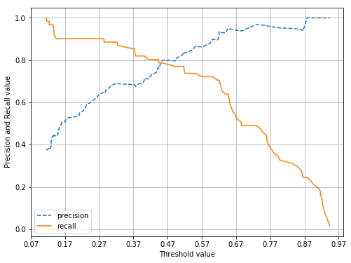

정밀도 점선, 재현율 실선
임곗값이 낮을수록 많은 수의 양성 예측으로 인해 재현율 값은 극도로 높아지고 정밀도는 극도로 낮아짐