
목차
- 장르 분석
1-1. 장르 선호도 전체적인 막대그래프 분석
1-2. 장르 선호도 히트맵
1-3. 장르 선호도 국가별 TOP3
1-4. 연도별 게임 출고량의 따른 장르 트렌드
1-5. 연도별 최고 판매량을 기록한 장르
- 플랫폼 분석
2-1. 플랫폼별 판매량 막대 그래프
2-2. 플랫폼별 판매량 TOP3
2-3. 년도별 출시량이 제일 많았던 플랫폼
2-4. 년도별 최고 판매량을 기록했던 플랫폼
-
게임회사 분석
3-1. 게임회사별 판매량
3-2. 년도별 최고 출시량을 기록한 회사
3-3. 년도별 최고 판매량을 기록한 회사 -
TOP10 게임 분석
4-1. 역대 판매량 TOP10 게임
4-2. 최근 10년 판매량 TOP10 게임
4-3. 최근 10년 TOP10 게임의 회사, 플랫폼, 장르의 판매량
결론
필요 패키지 import
import numpy as np
import pandas as pd
import matplotlib.pyplot as plt
import seaborn as sns
import warnings
warnings.filterwarnings('ignore')
%matplotlib inline
plt.rcParams['font.family'] = 'NanumGothic'
plt.rc('axes', unicode_minus=False)
%config InlineBackend.figure_format = 'retina'
1. 장르분석
1-1. 장르 선호도 전체적인 막대그래프 분석
temp_genre = df[['Genre', 'NA_Sales', 'EU_Sales', 'JP_Sales', 'Other_Sales']]
temp_genre.columns = ['장르', '미국 판매량', '유럽 판매량', '일본 판매량', '나머지 국가 판매량']
temp_grouped = temp_genre.groupby(['장르']).sum()
temp_table = temp_grouped.reset_index()

temp_table.columns = ['장르', '미국 판매량', '유럽 판매량', '일본 판매량', '나머지 국가 판매량']
temp_table.head()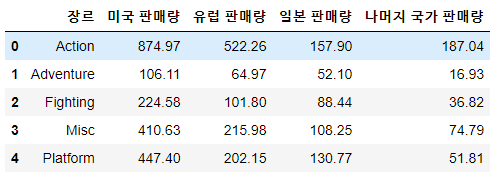
temp_melted = pd.melt(temp_table, id_vars=['장르'], value_vars=temp_table.columns[1:],
                      var_name='판매국가', value_name='판매량')
temp_melted.head()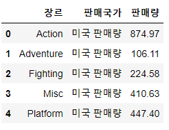
plt.figure(figsize=(16, 10))
sns.barplot(data=temp_melted, x='장르', y='판매량', hue='판매국가')
plt.title('국가별 장르 선호도', loc='center', fontsize=24)
plt.legend(fontsize=14)
plt.show()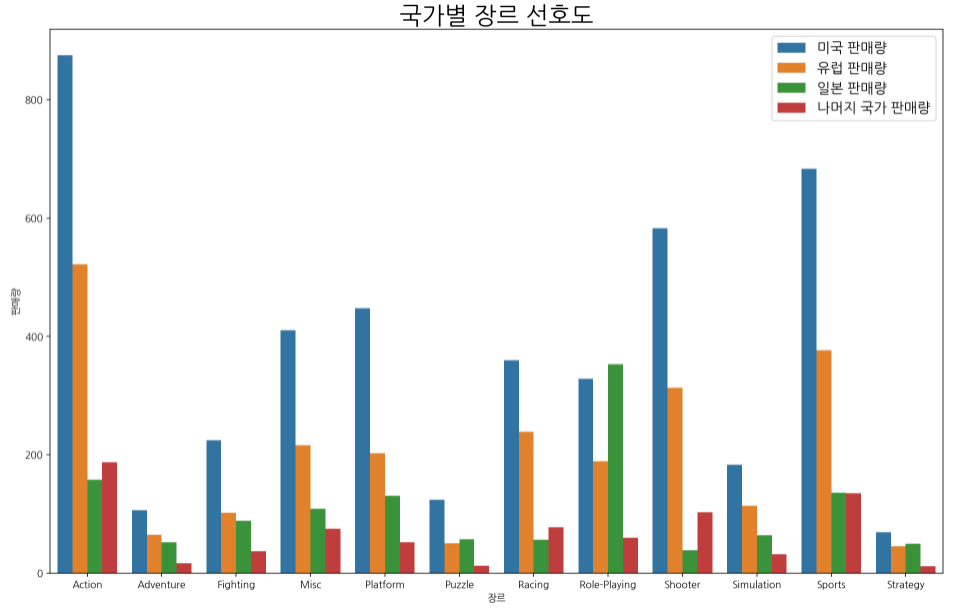
Action -> Sports -> Shooter 순으로 선호도가 보인다.
1-2. 장르 선호도 히트맵
plt.figure(figsize=(15, 10))

a = sns.heatmap(temp_grouped, annot=True, fmt = '.2f', cmap="YlGnBu")
plt.xticks(fontsize=14)
plt.yticks(fontsize=14)
a.set_ylabel('', fontsize=12)
plt.show()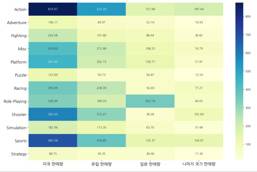
미국과 유럽의 선호도는 비슷한 형태를 띈다.
일본 같은 경우는 Role-Playing을 더 선호한다.
1-3. 장르 선호도 국가별 TOP3
# 국가별 판매량 TOP3
def top3_genre(df, sales_col):
    new_df = df.loc[:, ['장르', sales_col]].sort_values(by=sales_col, ascending=False).reset_index(drop=True).head(3)
    new_df.columns = ['장르', '판매량']
    return new_df

# Top3 데이터 저장
na_genre_top3 = top3_genre(temp_table, '미국 판매량')
eu_genre_top3 = top3_genre(temp_table, '유럽 판매량')
jp_genre_top3 = top3_genre(temp_table, '일본 판매량')
other_genre_top3 = top3_genre(temp_table, '나머지 국가 판매량')
# 데이터 리스트에 담기
data_list = [na_genre_top3, eu_genre_top3, jp_genre_top3, other_genre_top3]
columns_list = temp_table.columns[1:]
# 막대 그래프 그리기
fig, axs = plt.subplots(figsize=(26, 10), nrows=1, ncols=4)
for col, i, data in zip(columns_list, range(len(columns_list)), data_list):
    axs[i].set_title(col + ' ' + 'TOP3', fontsize=24)
    sns.barplot(x='장르', y='판매량', data=data, ax=axs[i])
    axs[i].tick_params(axis='both',labelsize=16)
    axs[i].set_xlabel('장르', fontsize=16)
    axs[i].set_ylabel('판매량', fontsize=16)
plt.show()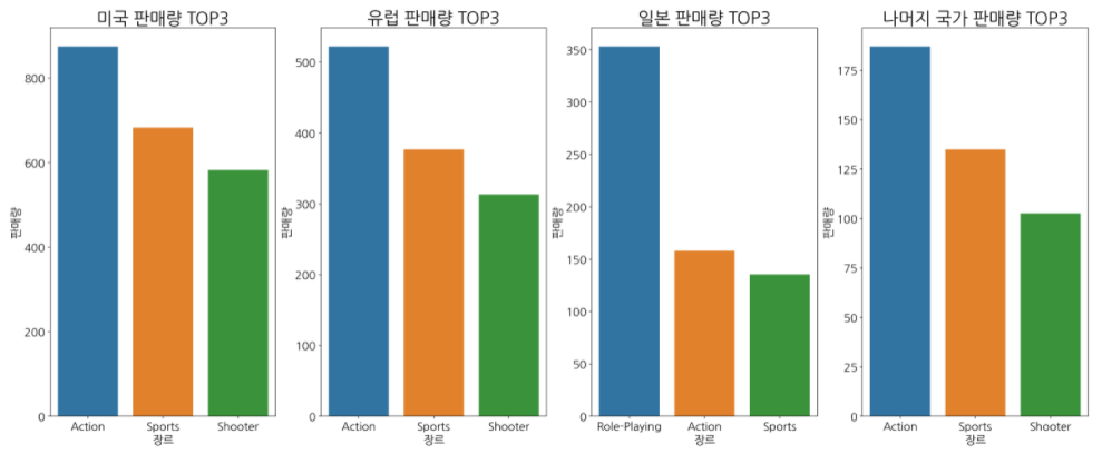
일본을 제외한 지역은 Action -> Sports -> Shooter 장르를 선호한다.
일본은 Role-Playing을 가장 선호하지만 그래도 Action-> Sports 장르도 선호하는 편이다.
전체적으로 Action 장르를 가장 선호한다고 볼 수 있다.
1-4. 연도별 게임 출고량의 따른 장르 트렌드
# 년도별 장르 갯수
year_max_df = df.groupby(['Year', 'Genre']).size().reset_index(name='count')
# 가장 값이 큰 값만 뽑기
year_max_idx = year_max_df.groupby(['Year'])['count'].transform(max) == year_max_df['count']
year_max_genre = year_max_df[year_max_idx].reset_index(drop=True)
# 중복값 제외하기
year_max_genre = year_max_genre.drop_duplicates(subset=['Year','count'], keep='last').reset_index(drop=True)
year_max_genre[:5]
year_max_genre.columns = ['년도', '장르', '출시량']

# 장르값 할당
genre = year_max_genre['장르'].values

# 년도별 최고 판매량 기록한 장르 데이터프레임 만들기
year_max_sales = df.groupby(['Year', 'Genre'])['Global_Sales'].sum().reset_index()
condition = year_max_sales['Global_Sales'] == year_max_sales.groupby(['Year'])['Global_Sales'].transform(max)
year_max_sales = year_max_sales[condition]
year_max_sales.columns = ['년도', '장르', '전세계 판매량']
year_max_sales[:5]

# 스타일 변경
sns.set_context('notebook')
sns.set_style('whitegrid')
plt.rcParams['font.family'] = 'NanumGothic'

plt.figure(figsize=(28,10))
ax = sns.barplot(x='년도', y='출시량', data=year_max_genre)
idx = 0
for value in year_max_genre['출시량']:
    ax.text(x=idx, y=value + 5, s=str(genre[idx] + '---' + ' ' + str(value)),
            color='black', size=14, rotation=90, ha='center')
    idx += 1
plt.xticks(rotation=90, fontsize=12)
plt.yticks(fontsize=12)
plt.xlabel('년도', fontsize=14)
plt.ylabel('출시량', fontsize=14)
ax.set_title('년도별 최고 출시량을 기록한 장르', fontsize=28, y=1.05, loc='left')
plt.show()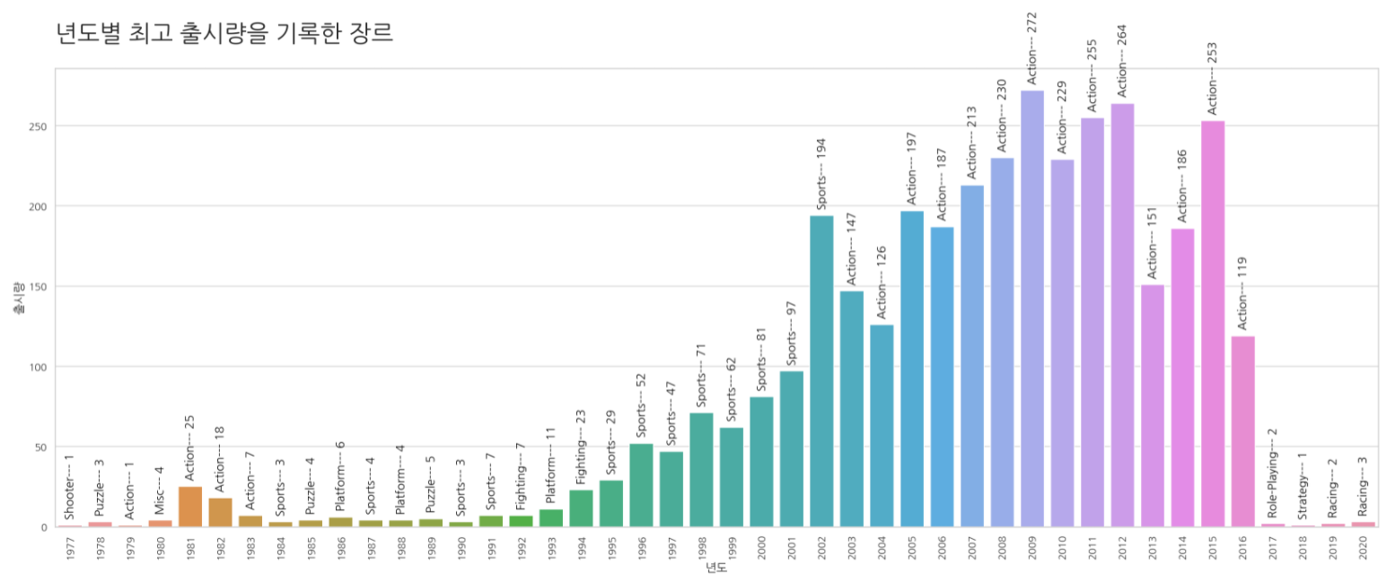
Action이 최근 트렌드였다고 볼 수 있다.
1-5. 연도별 최고 판매량을 기록한 장르
# 년도별 최고 판매량 기록한 장르 데이터프레임 만들기
year_max_sales = df.groupby(['Year', 'Genre'])['Global_Sales'].sum().reset_index()
condition = year_max_sales['Global_Sales'] == year_max_sales.groupby(['Year'])['Global_Sales'].transform(max)
year_max_sales = year_max_sales[condition]
year_max_sales.columns = ['년도', '장르', '전세계 판매량']

# 장르 데이터 저장
genre = year_max_sales['장르'].values

# 그래프 그리기
plt.figure(figsize=(28,10))
ax = sns.barplot(x='년도', y='전세계 판매량', data=year_max_sales)
idx = 0
for value in year_max_sales['전세계 판매량']:
    ax.text(x=idx, y=value + 2, s=str(genre[idx] + '---' + ' ' + str(round(value, 2))),
            color='black', size=14, rotation=90, ha='center')
    idx += 1
ax.set_title('년도별 최고 판매량을 기록한 장르', y=1.06, fontsize=28, loc='left')
plt.xticks(rotation=90, fontsize=12)
plt.yticks(fontsize=12)
plt.xlabel('년도', fontsize=16)
plt.ylabel('전세계 판매량', fontsize=16)
plt.show()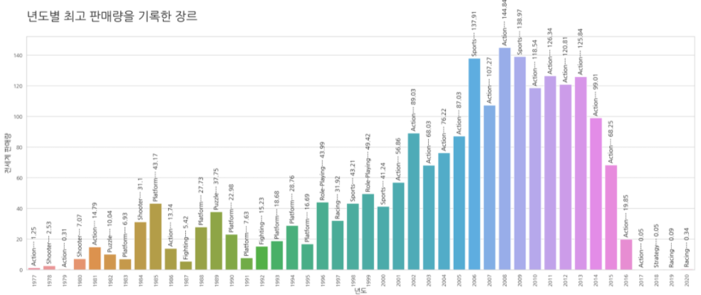
Action 장르가 트렌드를 탄 만큼 판매율을 보였다.
최종적으로 Action의 선호가 높다.
2. 플랫폼 분석
2-1. 플랫폼별 판매량 막대 그래프
# 지역별 플랫폼 선호도 분석
pf_by_sales = df[['Platform', 'NA_Sales', 'EU_Sales', 'JP_Sales', 'Other_Sales']]
pf_by_sales.columns = ['플랫폼', '미국 판매량', '유럽 판매량', '일본 판매량', '나머지 국가 판매량']
pf_by_sales_grouped = pf_by_sales.groupby(by=['플랫폼']).sum()
pf_by_sales_df = pf_by_sales_grouped.reset_index()
pf_by_sales_mt = pd.melt(pf_by_sales_df, id_vars=['플랫폼'], value_vars=pf_by_sales.columns[1:],
                         var_name='판매국가', value_name='판매량')

# pf_by_sales_mt

plt.figure(figsize=(28,10))
ax = sns.barplot(x='플랫폼', y='판매량', hue='판매국가', data=pf_by_sales_mt)
ax.set_title('플랫폼별 판매량', fontsize=28)
ax.legend(fontsize=16)
plt.xticks(fontsize=16)
plt.yticks(fontsize=16)
plt.show()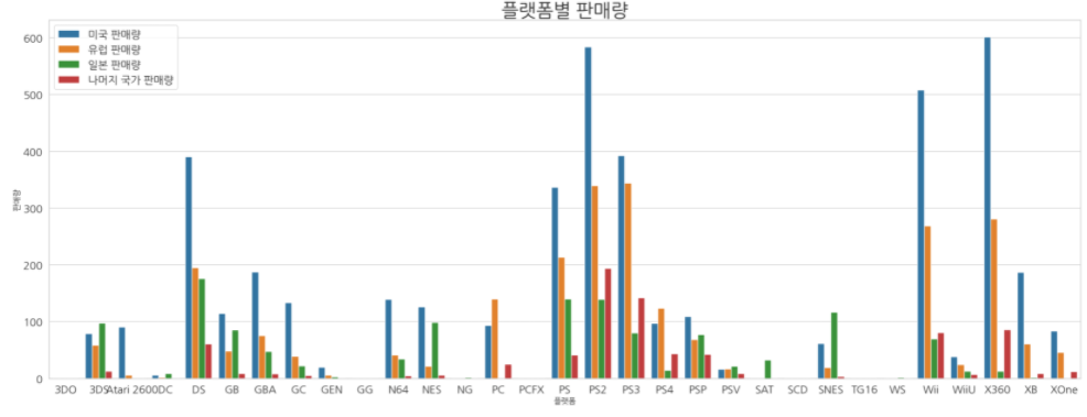
플레이스테이션은 전체적으로 선호도가 있는 편이고, 닌텐도는 wii, Ds
XBox는 x360모델이 가장 인기있다.
2-2. 플랫폼별 판매량 TOP3
def top3_platform(df, sales_col):
    new_df = df.loc[:, ['플랫폼', sales_col]].sort_values(by=sales_col, ascending=False).reset_index(drop=True).head(3)
    new_df.columns = ['플랫폼', '판매량']
    return new_df
na_platform_t3 = top3_platform(pf_by_sales_df, '미국 판매량')
eu_platform_t3 = top3_platform(pf_by_sales_df, '유럽 판매량')
jp_platform_t3 = top3_platform(pf_by_sales_df, '일본 판매량')
other_platform_t3 = top3_platform(pf_by_sales_df, '나머지 국가 판매량')

# 데이터 리스트에 담기
data_list = [na_platform_t3, eu_platform_t3, jp_platform_t3, other_platform_t3]
columns_list = pf_by_sales.columns[1:]
# 막대 그래프 그리기
fig, axs = plt.subplots(figsize=(28, 10), nrows=1, ncols=4)
for col, i, data in zip(columns_list, range(len(columns_list)), data_list):
    axs[i].set_title(col + ' ' + 'TOP3', fontsize=24)
    sns.barplot(x='플랫폼', y='판매량', data=data, ax=axs[i])
    axs[i].tick_params(labelsize=16)
    axs[i].set_xlabel('플랫폼', fontsize=16)
    axs[i].set_ylabel('판매량', fontsize=16)

plt.show()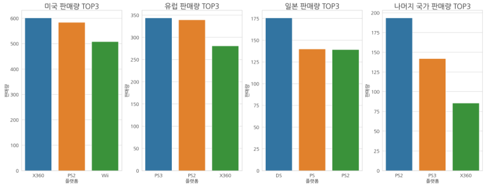
전체적으로 플레이스테이션의 선호도가 높다고 볼 수 있다.
2-3. 년도별 출시량이 제일 많았던 플랫폼
# 년도별 플랫폼 갯수
year_max_pf = df.groupby(['Year', 'Platform']).size().reset_index(name='count')
# 가장 값이 큰 값만 뽑기
condition = year_max_pf.groupby(['Year'])['count'].transform(max) == year_max_pf['count']
year_max_pf = year_max_pf[condition].reset_index(drop=True)
# 중복값 제외하기
year_max_pf = year_max_pf.drop_duplicates(subset=['Year','count'], keep='last').reset_index(drop=True)
year_max_pf.columns = ['년도', '플랫폼', '출시량']

# 플랫폼값 할당
platform = year_max_pf['플랫폼'].values

# 그래프 그리기
plt.figure(figsize=(28,10))
ax = sns.barplot(x='년도', y='출시량', data=year_max_pf)
idx = 0
for value in year_max_pf['출시량']:
    ax.text(x=idx, y=value + 5, s=str(platform[idx] + '---' + ' ' + str(value)),
            color='black', size=14, rotation=90, ha='center')
    idx += 1
plt.xticks(rotation=90, fontsize=12)
plt.yticks(fontsize=12)
plt.xlabel('년도', fontsize=14)
plt.ylabel('출시량', fontsize=14)
ax.set_title('년도별 최고 출시량을 기록한 플랫폼', fontsize=28, y=1.05, loc='left')
plt.show()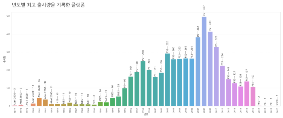
플레이스테이션이 시장을 점유하고 있다고 볼 수 있다.
2-4. 년도별 최고 판매량을 기록했던 플랫폼
# 년도별 최고 판매량 기록한 장르 데이터프레임 만들기
year_max_sales = df.groupby(['Year', 'Platform'])['Global_Sales'].sum().reset_index()
condition = year_max_sales['Global_Sales'] == year_max_sales.groupby(['Year'])['Global_Sales'].transform(max)
year_max_sales = year_max_sales[condition]
year_max_sales.columns = ['년도', '플랫폼', '전세계 판매량']
year_max_sales[:5]

# 플랫폼 값 저장
platform = year_max_sales['플랫폼'].values

#그래프 그리기
plt.figure(figsize=(28,10))
ax = sns.barplot(x='년도', y='전세계 판매량', data=year_max_sales)
idx = 0
for value in year_max_sales['전세계 판매량']:
    ax.text(x=idx, y=value + 2, s=str(platform[idx] + '---' + ' ' + str(round(value, 2))),
            color='black', size=14, rotation=90, ha='center')
    idx += 1
ax.set_title('년도별 최고 판매량을 기록한 플랫폼', y=1.06, fontsize=28, loc='left')
plt.xticks(rotation=90, fontsize=12)
plt.yticks(fontsize=12)
plt.xlabel('년도', fontsize=16)
plt.ylabel('전세계 판매량', fontsize=16)
plt.show()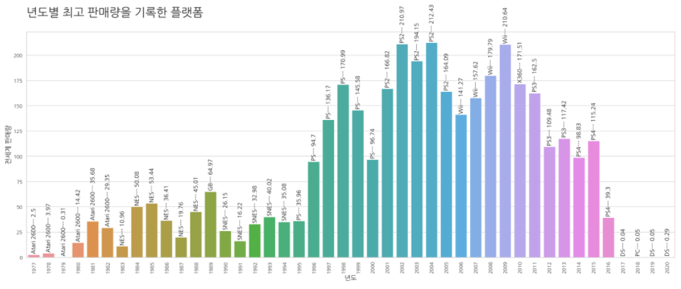
플레이스테이션이 출시도 많은 만큼 높은 판매량을 기록했다.
wii 같은 경우는 2006년 출시당시에 인기를 끌었지만, 플레이스테이션의 후속작으로 인해 시장에서 밀렸다. 결국 "플레이스테이션을 플랫폼으로 가장 선호한다." 라고 볼 수 있다.
3. 게임회사 분석
3-1. 게임회사별 판매량
# 게임 회사별 판매량 막대 그래프
publisher_by_sales = df[['Publisher', 'NA_Sales', 'EU_Sales', 'JP_Sales', 'Other_Sales', 'Global_Sales']]
publisher_by_sales.columns = ['회사명', '미국 판매량', '유럽 판매량', '일본 판매량', '나머지 국가 판매량', '전세계 판매량']

publisher_by_sales_grouped = publisher_by_sales.groupby(by=['회사명']).sum()

publisher_by_sales_df = publisher_by_sales_grouped.reset_index().sort_values(by=['전세계 판매량'], ascending=False).head(10)
publisher_by_sales_mt = pd.melt(publisher_by_sales_df, id_vars=['회사명'], value_vars=publisher_by_sales.columns[1:-1],
                         var_name='판매국가', value_name='판매량')


plt.figure(figsize=(28,10))
ax = sns.barplot(x='회사명', y='판매량', hue='판매국가', data=publisher_by_sales_mt)
ax.set_title('게임회사별 판매량', fontsize=28)
ax.tick_params(labelsize=14)
ax.legend(fontsize=14)
plt.show() 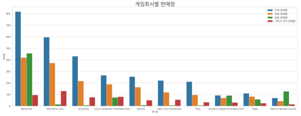
회사별 판매량 데이터를 보면 일본을 제외한 국가는 회사의 국적에 영향없이 선호도를 보인다. 하지만 일본 같은 경우는 자국 회사에 높은 선호도를 보이는 것으로 나타난다.
3-2. 년도별 최고 출시량을 기록한 회사
# 출시량 데이터 프레임 만들기
year_max_com = df.groupby(['Year', 'Publisher']).size().reset_index(name='count')
condition = year_max_com['count'] == year_max_com.groupby(['Year'])['count'].transform(max)
year_max_com = year_max_com[condition]
# year_max_com[:15]

# 중복값 제외하기
year_max_com = year_max_com.drop_duplicates(subset=['Year','count'], keep='last').reset_index(drop=True)
year_max_com.columns = ['년도', '회사명', '출시량']

# 회사명 값 저장
publisher = year_max_com.회사명

# 그래프 그리기
plt.figure(figsize=(28,10))
ax = sns.barplot(x='년도', y='출시량', data=year_max_com)
idx = 0
for value in year_max_com['출시량']:
    ax.text(x=idx, y=value + 5, s=str(publisher[idx] + '---' + ' ' + str(value)),
            color='black', size=14, rotation=90, ha='center')
    idx += 1
plt.xticks(rotation=90, fontsize=12)
plt.yticks(fontsize=12)
plt.xlabel('년도', fontsize=14)
plt.ylabel('출시량', fontsize=14)
ax.set_title('년도별 최고 출시량을 기록한 회사', fontsize=28, y=1.05, loc='left')
plt.show()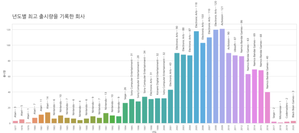
1990년도 후반에 일본회사들이 점유했지만, 곧 미국회사들이 점유했다.
2016년도 후반엔 Namco Bandai Games사의 게임이 가장 높은 출시량을 기록했다.
출시량들은 판매량에 영향을 미쳤을까?
3-3. 년도별 최고 판매량을 기록한 회사
# 회사의 년도별 판매량 데이터 프레임 만들기
year_sales_com = df.groupby(['Year', 'Publisher'])['Global_Sales'].sum().reset_index(name='sales')
condition = year_sales_com['sales'] == year_sales_com.groupby(['Year'])['sales'].transform(max)
year_sales_com = year_sales_com[condition]

# 중복값 마지막값이외에 제외하기
year_sales_com = year_sales_com.drop_duplicates(subset=['Year','sales'], keep='last').reset_index(drop=True)

year_sales_com.columns = ['년도', '회사명', '판매량']

publisher = year_sales_com.회사명


plt.figure(figsize=(28,10))
ax = sns.barplot(x='년도', y='판매량', data=year_sales_com)
idx = 0
for value in year_sales_com['판매량']:
    ax.text(x=idx, y=value + 5, s=str(publisher[idx] + '---' + ' ' + str(round(value, 2))),
            color='black', size=14, rotation=90, ha='center')
    idx += 1
plt.xticks(rotation=90, fontsize=12)
plt.yticks(fontsize=12)
plt.xlabel('년도', fontsize=14)
plt.ylabel('판매량', fontsize=14)
ax.set_title('년도별 최고 판매량을 기록한 회사', fontsize=28, y=1.05, loc='left')
plt.show()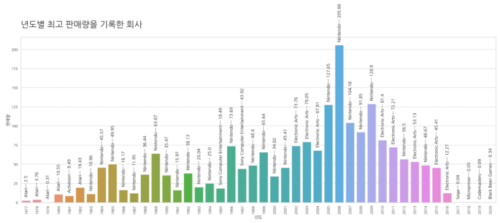
Namco Bandai Games의 출시량은 판매량에 영향을 끼치지 못했다.
1990년도 후반의 닌텐도사의 높은 출시량은 곧 높은 판매량으로 이어졌고,
Sony는 출시량에 비해 닌텐도 사에게 최고 판매량 자리를 내놓았다.
EA사의 이어지는 많은 출시량으로 판매량을 확보했고, 앞에서 보았던
닌텐도 wii의 높은 판매량이 닌텐도사에 영향이 있었다.
결국 회사가 큰 영향을 끼쳤다기보단 회사가 내놓은 게임 자체에 영향이 있었던 것 같다.
4. TOP10 게임 분석
4-1. 역대 판매량 TOP10 게임
# 판매량이 높은 Top10
sales_top10 = df.loc[df.Global_Sales.sort_values(ascending=False).index].reset_index(drop=True).head(10)
rank = [str(x)+' 위' for x in range(1, 11)]
sales_top10['rank'] = rank
sales_top10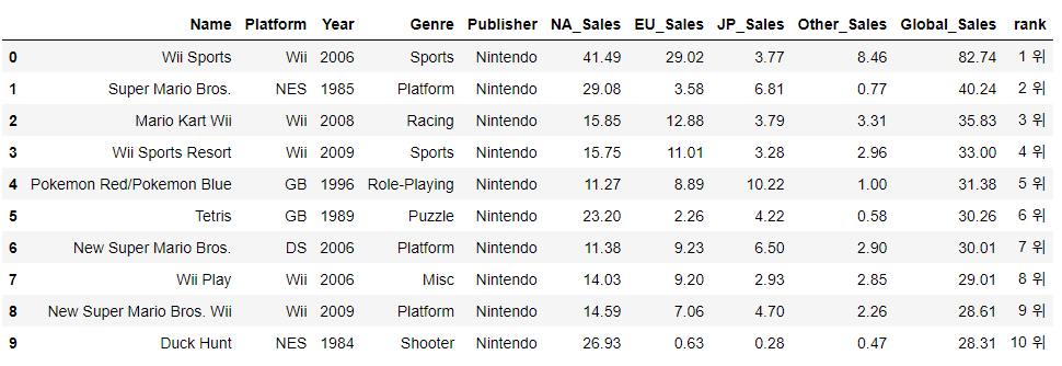
plt.figure(figsize=(32,10))
a = sns.barplot(x='rank', y='Global_Sales', data=sales_top10)
i = 0
for name, year, val, platform, publisher in zip(sales_top10.Name, sales_top10.Year, sales_top10.Global_Sales,
                                                sales_top10.Platform, sales_top10.Publisher):
    a.text(x=i, y=val+2, s=(name), color='black', ha='center', fontsize=15)
    a.text(x=i, y=val-8, s=(str(year) + '년' + '\n' + publisher + '\n' + platform), color='black', ha='center', fontsize=15)
    i+=1
a.set_title('판매량 역대 TOP10 게임', fontsize=28)
plt.xticks(fontsize=14)
plt.yticks(fontsize=14)
plt.xlabel('게임명', fontsize=16)
plt.ylabel('판매량', fontsize=16)
plt.show()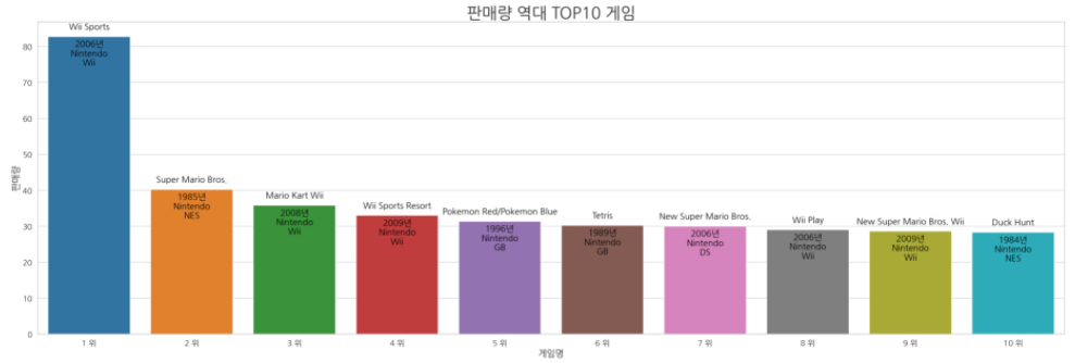
닌텐도 사가 역대 TOP10을 독점했다.
닌텐도 wii가 얼마나 인기가 있었는지 실감할 수 있었다.
그리고 유명한 고전게임인 테트리스도 있다.
중요한 것은 wii와 테트리스 등 고전 게임을 제외하면 마리오 시리즈와 포켓몬 시리즈가 눈에 보인다.
4-2. 최근 10년 판매량 TOP10 게임
year_sales_top_game = df[df.Year >= 2011].sort_values('Global_Sales', ascending=False).head(10)
year_sales_top_game = year_sales_top_game.reset_index(drop=True)
year_sales_top_game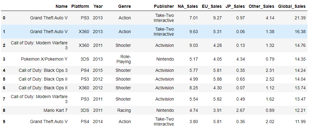
plt.figure(figsize=(32, 15))
a = sns.barplot(x = year_sales_top_game.index, y='Global_Sales', data=year_sales_top_game)
i = 0
for name, val in zip(year_sales_top_game.Name, year_sales_top_game.Global_Sales):
    if val >= 7:
        a.text(x=i, y=val-1, s=(name), ha='center',va='top', fontsize=28, rotation=90)
    else:
        a.text(x=i, y=val+1, s=(name), ha='center', fontsize=28, rotation=90)

    i+=1
a.set_title('최근 10년의 판매량 1위 게임', fontsize=30)
plt.xticks(ticks=[x for x in range(10)], labels=[str(x)+' 위' for x in range(1, 11)], fontsize=16)
plt.show()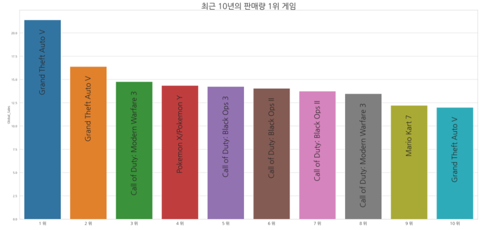
앞에서 봤던 역대 게임 TOP10에서도 마리오 포켓몬 시리즈가 있었다.
최근 2011~2020년의 데이터에서는 TOP10이 모두 시리즈 게임이다.
4-4. 최근 10년 TOP10 게임의 플랫폼, 장르의 판매량
def recent_year_Top3_sales(df, col, sales):
    return df.groupby(col)[sales].sum().reset_index(name='sales').sort_values('sales', ascending=False).head(3)

# 최근 10년 회사 판매량 Top3
# publisher_sales_top3 = recent_year_Top3_sales(year_sales_top_game, 'Publisher', 'Global_Sales')
# 최근 10년 플랫폼 판매량 Top3
platform_sales_top3 = recent_year_Top3_sales(year_sales_top_game, 'Platform', 'Global_Sales')
# 최근 10년 장르 판매량 Top3
genre_sales_top3 = recent_year_Top3_sales(year_sales_top_game, 'Genre', 'Global_Sales')

data_list = [platform_sales_top3, genre_sales_top3]
titles = ['최근 10년 판매량 1위 플랫폼 Top3', '최근 10년 판매량 1위 장르 Top3']
x_labels = ['플랫폼', '장르']

fig, axs = plt.subplots(figsize=(25,10), nrows=1, ncols=2)
for i, data, title in zip(range(3), data_list, titles):
    sns.barplot(x=data.iloc[:,0], y=data.iloc[:,1], ax=axs[i])
    axs[i].set_title(titles[i], fontsize=20)
    axs[i].tick_params(labelsize=14)
    axs[i].set_xlabel(x_labels[i], fontsize=16)
    axs[i].set_ylabel('판매량', fontsize=16)
plt.show()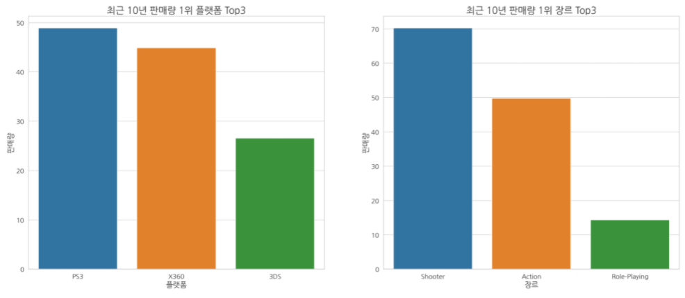
최근 판매량 TOP10의 플랫폼을 확인해보니 역시나 1위는 플레이스테이션이었다.
장르 같은 경우 call of duty가 Shooter 장르로 분류되고, GTA는 사실상 Action Adventure다 call of duty는 시리즈가 너무 유명하고 인기가 있기 때문에 결론에 영향을 주진 않았다.
결론
다음 분기에 어떤 게임을 설계해야 할까?
플레이스테이션을 플랫폼으로 한 액션 장르의 시리즈물을 설계하는 것이 좋을 것 같다.

2개의 댓글

The main thing in a bookmaker is reliability, and https://melbetapk-mo.com/ is showing its best side so far. The line is wide, the coefficients are normal, and the site is working smoothly. Live bets are accepted quickly. Winnings are paid out without delay. It's a great option so far.
Ethan was fascinated by roulette but had always felt intimidated by its complexity. To overcome this, he decided to start with a basic European roulette https://goldenpokiescasino1.com/ game online. With a modest bankroll and an open mind, Ethan explored different betting strategies, from simple even-money bets to more complex ones like the Martingale system. His initial sessions were a mix of ups and downs, but he approached each spin with curiosity and a desire to learn.