[TIL] 21.06.10 Ridge Regression

1. pandas_profiling.ProfileReport

from pandas_profiling import ProfileReport

ProfileReport(df)
# 데이터 프레임의 전체적인 내용을 보여줌

2. Ridge Regression

캐글의 Melbourne Housing Market 를 사용

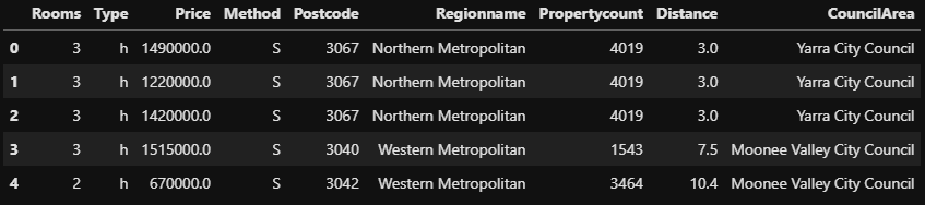
# 필요한 모듈 import
import pandas as pd
from sklearn.model_selection import train_test_split
from category_encoders import OneHotEncoder
from sklearn.feature_selection import f_regression, SelectKBest
from sklearn.linear_model import RidgeCV, Ridge
import matplotlib.pyplot as plt
import seaborn as sns
%matplotlib inline
import warnings
warnings.filterwarnings('ignore')

df.head()

전처리를 진행하고 회귀에 필요한 데이터만 가져와서 진행

2-1. 우편번호 범주형 변환

# 우편번호의 데이터 확인
df.Postcode.value_counts()
#
# out:
# 3073    802
# 3020    649
# 3046    641
# 3064    626
# 3150    625
#        ... 
# 3767      1
# 3791      1
# 3788      1
# 3770      1
# 3781      1
# Name: Postcode, Length: 221, dtype: int64

2-2. One Hot Encoding

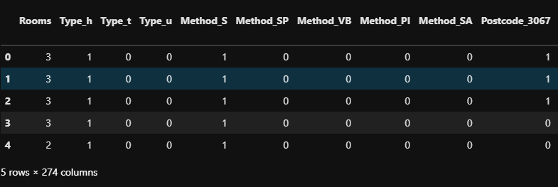
# Postcode는 우편번호로써 데이터 프레임에서 확인해보니 명목척도로 사용할 수 있다고 판단하여 string 변환
house = df.copy()
house['Postcode'] = house['Postcode'].astype(str)

# one hot encoding
encoder = OneHotEncoder(use_cat_names=True)
X = encoder.fit_transform(house.drop('Price', axis=1))
y = house[['Price']]
X.head()

2-3. 학습, 테스트 데이터 나누기

# 학습, 테스트 데이터 나누기
X_train, X_test, y_train, y_test = train_test_split(X, y, train_size=0.75, random_state=42)
#
# out:
# ((31886, 274), (10629, 274))

2-4. Feature Selection

# feature selection 30개의 feature만 선택

# Selector 정의
selector = SelectKBest(score_func=f_regression, k=30)

# 학습데이터에 fit_transform
X_train_selected = selector.fit_transform(X_train, y_train)

# 테스트데이터는 transform
X_test_selected = selector.transform(X_test)

X_train_selected.shape, X_test_selected.shape

#
# out:
# ((31886, 30), (10629, 30))

# 전체 컬럼 가져오기
all_col = X_train.columns

# 선택된 컬럼 boolean (선택된 것은 True, 선택되지 않은 것은 False)
col_mask = selector.get_support()

# 선택된 컬럼만 가져오기
use_col = all_col[col_mask]

use_col

#
# out:
# Index(['Rooms', 'Type_h', 'Type_u', 'Method_SP', 'Method_VB', 'Postcode_3206',
#        'Postcode_3103', 'Postcode_3104', 'Postcode_3186', 'Postcode_3187',
#        'Postcode_3124', 'Postcode_3126', 'Postcode_3064', 'Postcode_3146',
#        'Postcode_3101', 'Postcode_3144', 'Postcode_3127', 'Postcode_3142',
#        'Regionname_Northern Metropolitan', 'Regionname_Western Metropolitan',
#        'Regionname_Southern Metropolitan', 'Distance',
#        'CouncilArea_Brimbank City Council',
#        'CouncilArea_Stonnington City Council',
#        'CouncilArea_Boroondara City Council',
#        'CouncilArea_Bayside City Council', 'CouncilArea_Hume City Council',
#        'CouncilArea_Melton City Council',
#        'CouncilArea_Whittlesea City Council',
#        'CouncilArea_Wyndham City Council'],
#       dtype='object')

2-6. Selected Feature score

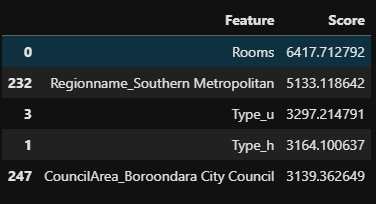
# feature별 점수 가져오기
f_score = selector.scores_
# 모든 컬럼 가져오기
f_name = X_train.columns
# Feature, score 항목으로 데이터 프레임 만들기
scores_df = pd.DataFrame(data={'Feature' : f_name, 'Score' : f_score})
# NaN 값이 있어서 drop
scores_df.dropna(inplace=True)
# Score 기준으로 정렬
scores_df = scores_df.sort_values('Score', ascending=False)
scores_df.head()

2-7. Selected Feature score visualization

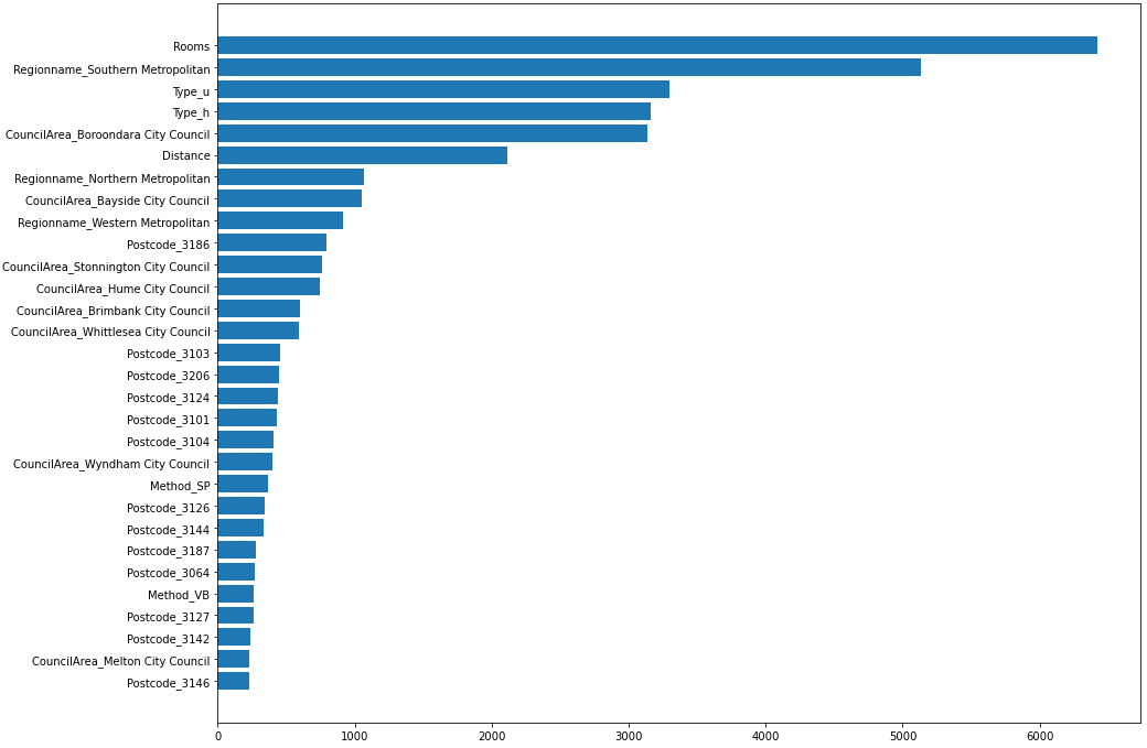
# TOP 30
plot_df = scores_df[:30]
# 시각화
plt.figure(figsize=(15, 12))
plt.barh(y=plot_df['Feature'], width=plot_df['Score'])
plt.gca().invert_yaxis() # 역정렬 문제 해결

plt.show()

Unselected feature drop

# 선택된 30개의 특성 외의 컬럼 drop
unuse_col = all_col[~col_mask]
# X_train.drop(unuse_col, axis=1, inplace=True)
# X_test.drop(unuse_col, axis=1, inplace=True)
# X_train.head()
# drop해서 score를 보았더니 drop하지 않은 모델이 더 성능이 좋았음

2-8. selected alpha

# 적용할 alpha값
alphas = [0, 0.001, 0.05, 0.01, 0.5, 0.1, 1, 1.5, 5, 10]

for alpha in alphas:
    # alpha값 모델에 적용
    model = Ridge(alpha=alpha, normalize=True, random_state=42)
    # 모델 훈련
    model.fit(X_train, y_train)
   
    # 만들어진 모델의 예측
    y_pred = model.predict(X_test)
    train_y_pred = model.predict(X_train)
    # MAE
    train_mae = mean_absolute_error(y_train, train_y_pred)
    mae = mean_absolute_error(y_test, y_pred)
    # R2 score
    train_score = r2_score(y_train, train_y_pred)
    score = r2_score(y_test, y_pred)
    print(f"alpha값 : {alpha} 의 모델")
    print(f"train MAE : {train_mae}")
    print(f"test MAE : {mae}")
    print(f"train r2score : {train_score}")
    print(f"test r2score : {score}")
    print('-'*50)
  
#
# out:
# alpha값 : 0 의 모델
# train MAE : 233334.2128520354
# test MAE : 3162521912267468.5
# train r2score : 0.6274332036924364
# test r2score : -8.326821060424468e+22
# --------------------------------------------------
# alpha값 : 0.001 의 모델
# train MAE : 233357.04625835957
# test MAE : 236702.22829697252
# train r2score : 0.6274333997631953
# test r2score : 0.620970993111954
# --------------------------------------------------
# alpha값 : 0.05 의 모델
# train MAE : 231681.71407159735
# test MAE : 234828.06149510358
# train r2score : 0.625944726321348
# test r2score : 0.6198416619265564
# --------------------------------------------------
# alpha값 : 0.01 의 모델
# train MAE : 233007.80566520247
# test MAE : 236255.28958365004
# train r2score : 0.6271481314360778
# test r2score : 0.6208968686468163
# --------------------------------------------------
# alpha값 : 0.1 의 모델
# train MAE : 230601.8480078
# test MAE : 233743.78119396255
# train r2score : 0.6236844572047637
# test r2score : 0.6175898367441484
# --------------------------------------------------
# alpha값 : 0.5 의 모델
# train MAE : 234883.21860835422
# test MAE : 237730.4567901982
# train r2score : 0.5887741959002399
# test r2score : 0.5829455475022739
# --------------------------------------------------
# alpha값 : 1 의 모델
# train MAE : 250755.35792173276
# test MAE : 253372.54580131633
# train r2score : 0.5364460041737951
# test r2score : 0.5313444128080818
# --------------------------------------------------
# alpha값 : 1.5 의 모델
# train MAE : 267522.8371968396
# test MAE : 269874.1750990744
# train r2score : 0.4887483315327904
# test r2score : 0.48430157947078956
# --------------------------------------------------
# alpha값 : 5 의 모델
# train MAE : 336856.90344772674
# test MAE : 339432.97196062293
# train r2score : 0.29397193200244265
# test r2score : 0.29169025809778315
# --------------------------------------------------
# alpha값 : 10 의 모델
# train MAE : 370704.4707108561
# test MAE : 373534.2665702095
# train r2score : 0.1862406767782282
# test r2score : 0.18487713753153534
# --------------------------------------------------

2-9. Select alpha with RidgeCV

# Ridge CV로 최적의 람다값 찾기

ridge = RidgeCV(alphas=alphas, normalize=True, cv=10)
ridge.fit(X_train, y_train)
print(f"alpha : {ridge.alpha_}")
print(f"best score : {ridge.best_score_}")

#
# out:
# alpha : 0.001
# best score : 0.6220519062358998

2-10. train model with optimal alpha

# Train model with optimal alpha
model = Ridge(alpha=0.001, normalize=True, random_state=42).fit(X_train, y_train)
# alpha = 0.001인 ridge회귀모델의 점수
train_score = model.score(X_train, y_train)
test_score = model.score(X_test, y_test)

print(f"train score : {train_score}")
print(f"test score : {test_score}")

#
# out:
# train score : 0.6274333997631953
# test score : 0.620970993111954

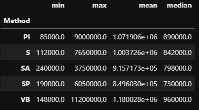
3. 범주형 데이터 형태 비교

df.groupby('Method')['Price'].agg(['min', 'max', 'mean', 'median'])

ETC

📌Data 분석 전체적인 흐름

*Data 간의 상관관계가 높았을 경우 처리 방법

0. EDA
   -시각화

1. 전처리

• 결측치, target 지정, 분포확인(mean, std)
• 통계적 지식이 필요한 부분 ( Scale은 이 부분에 해당되지 않는다)

2. 상관관계

• feature들 간의 상관관계
• target 값과의 분산확인
• density plot

3. 다중 회귀분석

• 독립변수들의 유의확률 값을 보았을 때, 다중공선성이 의심된다

4. 다중 공선성 진단

• 입력변수들 간의 상관정도가 높은 상태를 말한다.

5. 변수 선택법

• PCA
• select K best
• regression
• random forest(XGboost)
• feature importance
• permutation
• Ridge/lasso/elasticnet regression

6. 다중회귀를 통한 재검증

• 학습

7. train_test set 으로 분리

8. 모델에 학습시킨다(sacle 과정 필요)

9. 결과 값 확인

-R^2
-p-value
-confusion matrix

10. predict

📌Type of error

TP : 약이 효과가 있는데 있다고 판단
TN : 약이 효과가 없는데 없다고 판단
FP : 약이 효과가 없는데 있다고 판단
FN : 약이 효과가 있는데 없다고 판단