등장 횟수 기반의 단어 표현(Count-based Representation)
단어가 특정 문서에 들어있는 횟수를 바탕으로 벡터화 하는 방법이다.
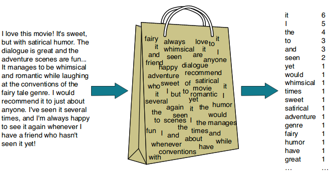
대표적인 방법으로는 Bag-of-Words(TF, TF-IDF)가 있다.
- 문서-단어 행렬(Document-Term Matrix, DTM)
벡터화 된 문서는 문서-단어 행렬의 형태로 나타나게 된다.
문서-단어 행렬이란 각 행에는 문서((Document)가, 각 열에는 단어(Term)가 있는 행렬이다.
| / | Word_1 | Word_2 | Word_3 | Word_4 | Word_5 |
|---|---|---|---|---|---|
| doc1 | 0 | 1 | 0 | 1 | 2 |
| doc2 | 1 | 0 | 0 | 1 | 1 |
| doc3 | 0 | 1 | 1 | 1 | 0 |
1. Bag-of-Words(BoW) : TF(Term Frequency)
가장 단순한 벡터화 방법 중 하나이다.
문서에서 단순히 단어들의 빈도만 고려하여 벡터화 하는 방법이다.
CounterVectorizer
# 예제 텍스트
text = """In information retrieval, tf–idf or TFIDF, short for term frequency–inverse document frequency, is a numerical statistic that is intended to reflect how important a word is to a document in a collection or corpus.
It is often used as a weighting factor in searches of information retrieval, text mining, and user modeling.
The tf–idf value increases proportionally to the number of times a word appears in the document and is offset by the number of documents in the corpus that contain the word,
which helps to adjust for the fact that some words appear more frequently in general.
tf–idf is one of the most popular term-weighting schemes today.
A survey conducted in 2015 showed that 83% of text-based recommender systems in digital libraries use tf–idf."""
# 문장별로 나눔
sentences = text.split('\n')
vect = CountVectorizer()
# 어휘 사전 생성
vect.fit(sentences)
vect.vocabulary_{'in': 26, 'information': 28, 'retrieval': 49, 'tf': 60, 'idf': 24,
'or': 44, 'tfidf': 61, 'short': 52, 'for': 18, 'term': 58,
'frequency': 19, 'inverse': 30, 'document': 14,
'is': 31, 'numerical': 39, 'statistic': 55, 'that': 62, 'intended': 29,
'to': 65, 'reflect': 48, 'how': 23, 'important': 25, 'word': 73,
'collection': 9, 'corpus': 12, 'it': 32, 'often': 42, 'used': 68,
'as': 6, 'weighting': 71, 'factor': 17, 'searches': 51, 'of': 40,
'text': 59, 'mining': 34, 'and': 3, 'user': 69, 'modeling': 35,
'the': 63, 'value': 70, 'increases': 27, 'proportionally': 46, 'number': 38,
'times': 64, 'appears': 5, 'offset': 41, 'by': 8,
'documents': 15, 'contain': 11, 'which': 72, 'helps': 22, 'adjust': 2, 'fact': 16,
'some': 54, 'words': 74, 'appear': 4, 'more': 36, 'frequently': 20, 'general': 21,
one': 43, 'most': 37, 'popular': 45, 'schemes': 50, 'today': 66, 'survey': 56,
'conducted': 10, '2015': 0, 'showed': 53, '83': 1, 'based': 7, 'recommender': 47,
'systems': 57, 'digital': 13, 'libraries': 33, 'use': 67}# text를 DTM(document-term matrix)으로 변환
dtm_count = vect.transform(sentences)
dtm_count = pd.DataFrame(dtm_count.todense(), columns=vect.get_feature_names())
dtm_count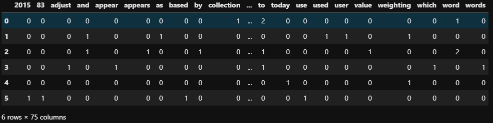
문장당 단어별 표현된 횟수를 나타내는 행렬을 볼 수 있다.
2. Bag-of-Words(BoW) : TF-IDF (Term Frequency - Inverse Document Frequency)
TF-IDF는 특징 추출 기법으로써 모델 학습시 변수를 만들 때 데이터의 특징을 담아서 학습시켜야 하기 때문에 사용된다. 텍스트 데이터를 벡터화 할 때 등장 횟수 기반의 단어 표현의 한계점을 해결하기 위해서 여러 문서에서 많이 등장하는 단어에 가중치를 적게 주어 큰 특징이 없지만 자주 등장하는 단어가 설명력이 높아지는 것을 방지한다.
TF-IDF의 식
-
TF(Term Frequency)
1개 문서 안에서 특정 단어의 등장 빈도를 의미한다.
1글자는 빈도수에서 제외된다. -
DF(Document Frequency)
특정 단어가 나타나는 문서 수를 의미한다.
즉 문서 3개에서 'bag'이란 단어가 전체 문서에서 6번 쓰였지만 나타난 총 문서 수는 2라면 DF=2이다. -
IDF(Inverse Document Frequency)
DF에 역수변환을 해준 값이다.
즉 역수를 취해주어 큰 값이 작은 값으로 줄어드는 효과를 이용해 많이 등장하는 단어에 페널티를 줄 수 있다.
from sklearn.feature_extraction.text import TfidfVectorizer
# TF-IDF vectorizer. 테이블을 작게 만들기 위해 max_features=15로 제한
tfidf = TfidfVectorizer(stop_words='english', max_features=15)

# Fit 후 dtm을 만든다.(문서, 단어마다 tf-idf 값을 계산)
dtm_tfidf = tfidf.fit_transform(sentences)

dtm_tfidf = pd.DataFrame(dtm_tfidf.todense(), columns=tfidf.get_feature_names())
dtm_tfidf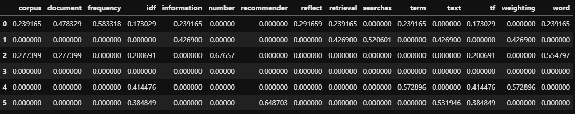

조금씩 천천히