🏷️ OpenCV Seed Counter 깃허브 링크
📚 Seed Counter
씨앗을 카운트하기 위해 만들어진 코드, 카메라로 찍은 씨앗 사진을 흑백으로 만든 뒤 명암의 범위를 설정하여 씨앗 윤곽선 부분만 검출, 검출된 씨앗의 윤곽선의 수를 카운트하여 값을 반환해주는 코드입니다.
📄 베이스 코드
iimport cv2
import numpy as np
import copy

image = cv2.imread('SEED_COUNTER\seed_count_image.jpg')
gray = cv2.cvtColor(image, cv2.COLOR_BGR2GRAY)
_, thresh = cv2.threshold(gray, 120, 255, cv2.THRESH_BINARY)

thresh = cv2.bitwise_not(thresh)
contours, _ = cv2.findContours(thresh, cv2.RETR_EXTERNAL, cv2.CHAIN_APPROX_SIMPLE)

result_image = copy.deepcopy(image)
result_image [thresh == 0] = [255, 255, 255]
cv2.drawContours(result_image, contours, -1, (0, 255, 0), 2)

contour_count = len(contours)
font = cv2.FONT_HERSHEY_SIMPLEX
cv2.putText(result_image, f"seed count: {contour_count}", (10, 30), font, 1, (0, 0, 255), 2)

cv2.imshow('Contours', result_image)
cv2.waitKey(0)
cv2.destroyAllWindows()
해당 코드에서는 저장된 이미지를 통해 시드를 카운트하는 코드로 가장 기본이 되는 베이스 코드입니다.
ㅤ
📕 임계값
이미지에서 특정한 색상이나 밝기의 영역만을 선택하기 위해 임계값(threshold)을 사용합니다. OpenCV에서는 cv2.threshold 함수를 사용하여 이진화 처리를 할 수 있으며, 이를 통해 배경과 객체를 분리할 수 있습니다. 또한, cv2.adaptiveThreshold를 사용하여 국소적인 영역에 따라 임계값을 다르게 적용할 수 있습니다. 이는 빛의 조건이 일정하지 않은 이미지에 유용합니다.ㅤ
image = cv2.imread('./seed_count_image.jpg')
gray = cv2.cvtColor(image, cv2.COLOR_BGR2GRAY)
_, thresh = cv2.threshold(gray, 120, 255, cv2.THRESH_BINARY)
이미지를 불러온 뒤 그레이스케일로 변환, 밝기 120을 임계값으로 설정하고 그 이상의 구역을 흰색(255)으로 변환하겠습니다.
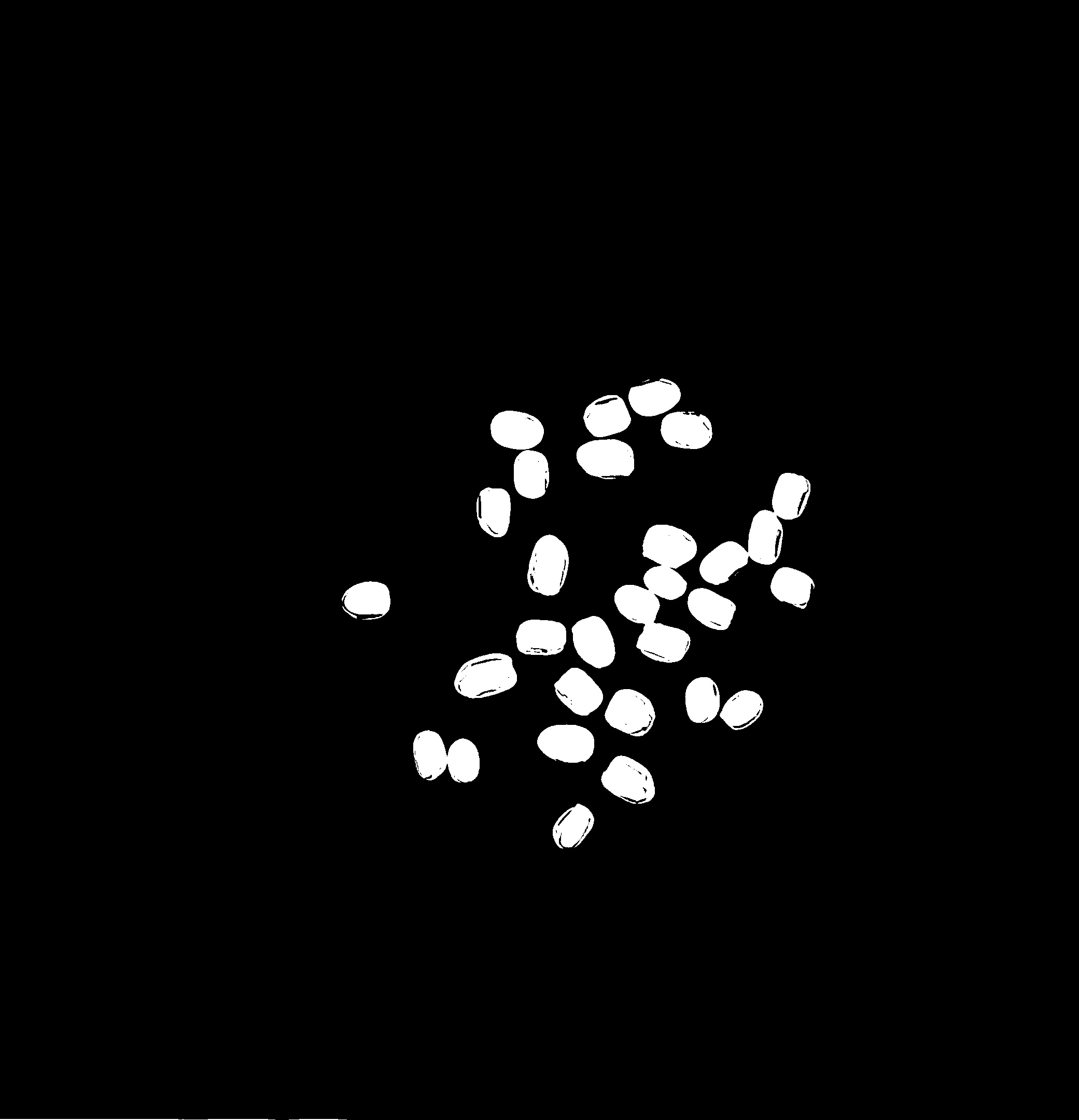
| cv2.bitwise_not을 통해 색반전 이전의 thresh | cv2.bitwise_not을 통해 색반전 이후의 thresh |
 |
 |
📕 윤곽선
윤곽선 분리는 이미지에서 객체의 외곽선을 찾아내는 과정입니다. 이를 통해 객체의 형태, 크기, 위치 등을 파악할 수 있으며, 이미지 분석, 객체 인식, 이미지 분할 등 다양한 분야에서 활용됩니다.
📙 윤곽선 검출
thresh = cv2.bitwise_not(thresh)
contours, _ = cv2.findContours(thresh, cv2.RETR_EXTERNAL, cv2.CHAIN_APPROX_SIMPLE)
cv2.findContours 함수는 이미지에서 흰색과 검은색의 경계를 윤곽선으로 간주하여 검출합니다. 윤곽선 검출을 위해서는 cv2.threshold를 통해 이미지를 이진화 처리하였으므로 이미지에서 윤곽선을 검출할 수 있습니다.
result_image = copy.deepcopy(image)
result_image [thresh == 0] = [255, 255, 255]
cv2.drawContours(result_image, contours, -1, (0, 255, 0), 2)
원본 이미지를 deepcopy를 통해 result_image를 생성, thresh의 검은색(0)부분을 흰색(255)로 변경한 뒤 result_image에 윤곽선을 그립니다.
📙 윤곽선 카운트
contour_count = len(contours)
font = cv2.FONT_HERSHEY_SIMPLEX
cv2.putText(result_image, f"seed count: {contour_count}", (10, 30), font, 1, (0, 0, 255), 2)
coutours의 갯수를 cv2.putText를 이용해 result_image에 표시해준다.
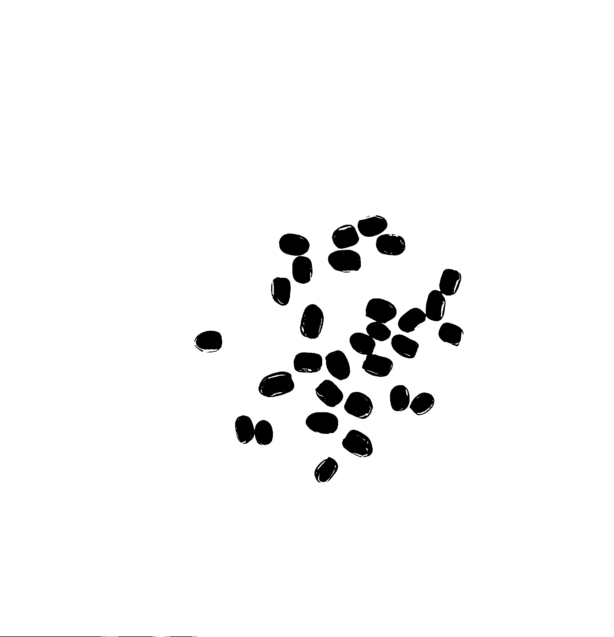
전체 코드를 실행할 경우 다음과 같은 이미지 출력된다.
 |
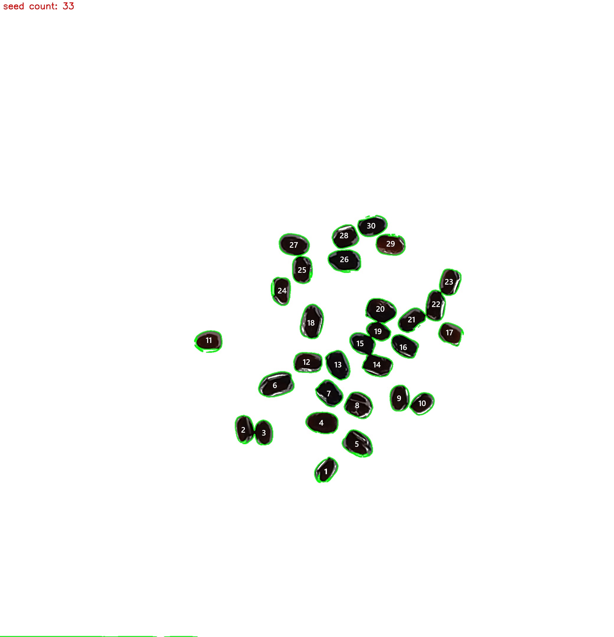
이미지 속 Seed의 실제 갯수는 30개로 3개의 오차가 발생한다. 이러한 오차가 발생하는 이유를 알기 위해선 어떤 윤곽선에서 문제가 발생하는지 알아볼 필요가 있습니다.
이를 확인하기 위해선 카운트된 윤곽선의 갯수를 이미지에 그려주는 코드를 추가합니다.
for i, contour in enumerate(contours):
    M = cv2.moments(contour)
    if M["m00"] != 0:
        cX = int(M["m10"] / M["m00"])
        cY = int(M["m01"] / M["m00"])
        cv2.putText(result_image, str(i + 1), (cX, cY), font, 1, (0, 0, 255), 2)
추가된 코드를 실행시키면 예상하지 못한 윤곽선이 카운트되거나 뭉쳐서 인식된 것을 볼 수 있습니다.
| 정상 카운트 된 부분 | 코드에서 카운트 된 부분 |
 |
 |
📕 윤곽선 넓이 필터
윤곽선 면적 계산 함수 cv2.contourArea는 단일 윤곽선의 면적을 계산합니다. 윤곽선을 인자로 받아 그 면적을 픽셀 단위로 반환합니다. 이를 통해 특정 면적 이상 또는 이하의 윤곽선을 필터링할 수 있습니다.
def filter_contours_by_size(self, contours: np.ndarray, min_area: int = 100, max_area: int = 1000) -> list:
    """
    주어진 윤곽선 목록에서 면적이 min_area와 max_area 사이인 윤곽선만을 필터링합니다.

    Args:
    - contours: np.ndarray, 윤곽선 목록
    - min_area: int, 필터링할 최소 면적 기준값
    - max_area: int, 필터링할 최대 면적 기준값

    Returns:
    - list: min_area와 max_area 사이의 면적을 가진 윤곽선 목록
    """
    filtered_contours = [contour for contour in contours if min_area <= cv2.contourArea(contour) <= max_area]
    return filtered_contours
filter_contours_by_size를 사용하게 되면 사용자가 원하는 크기 범위의 윤곽선만 출력이 가능하며 이를 통해 필요없는 부분의 윤곽선을 제외 시킬 수 있습니다. 일단 값을 100과 1000으로 잡고 실행시켜 카운트 된 갯수만 츨력해 보겠습니다
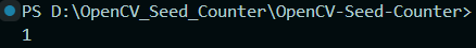
값이 1로 나왔습니다. 이는 윤곽선의 크기를 제대로 고려하지 않고 임의로 크기를 지정하여 발생한 것으로 기존 윤곽선과 필터 윤곽선의 넓이를 각각 출력하여 확인해 보겠습니다.
def Area_contours(self, contours: np.ndarray) -> None:
"""
윤곽선의 넓이를 계산하여 리스트에 할당합니다.
Args:
- contours: 윤곽선 목록
"""
self.areas = [cv2.contourArea(c) for c in contours] 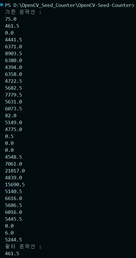 확인 결과 100과 1000 사이 크기를 가진 윤곽선은 1개이므로 카운트되 값 또한 1이 되는것이 맞았습니다.
그럼 문제를 파악했으니 윤곽선 리스트를 직접 확인하는 수작업 없이 윤곽선을 카운트 하도록 수정해 보겠습니다.
📙 중앙값으로 계산
def median_value_contours(self) -> float:
    """
    중앙값을 찾습니다.

    Returns:
    - median_value: 중앙값
    """
    median_value = np.median(self.areas)
    return median_value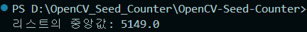
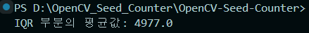
📙 IQR으로 계산
IQR(Interquartile Range, 사분위수 범위)은 데이터의 중간 50%에 해당하는 범위로, 제1사분위수(Q1)와 제3사분위수(Q3) 사이 범위를 의미합니다.
- 제1사분위수는 25th percentile, 전체 자료의 1/4 아래 있을 때의 지점
- 제3사분위수는 75th percentile, 전체 자료의 3/4 아래 있을 때의 지점
def IQR_value_contours(self) -> float:
    """
    IQR범위의 평균값을 찾습니다.

    Returns:
    - iqr_mean: IQR범위의 평균값
    """
    Q1 = np.percentile(self.areas, 25)
    Q3 = np.percentile(self.areas, 75)
    # IQR 범위에 해당하는 값들 필터링
    iqr_values = [x for x in self.areas if Q1 <= x <= Q3]
    # IQR 부분의 평균값 계산
    iqr_mean = np.mean(iqr_values)
    return iqr_mean
두가지 방법 중 어느 것을 고를지는 사용자의 마음이며 저는 비교적 코드상 가벼운 중앙값을 가지고 윤곽선을 필터링 해보겠습니다.
if __name__ == "__main__":
    SC = SeedC('./seed_count_image.jpg')
    contours = SC.find_contours()
    SC.Area_contours(contours)
    value = SC.median_value_contours()
    filter_contours = SC.filter_contours_by_size(contours, value*0.3, value*1.7)
    print(f"seed count: {len(filter_contours)}"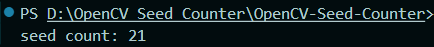
 출력값이 21이 나왔습니다. 기존에 작은 윤곽선은 카운트되지 않아 값이 기존보다 많이 카운트되진 않았지만 여전히 30개를 카운트하진 못했습니다.
이 다음 방법으로는 이미지에 씨앗이 서로 붙어 있는 부분을 워터셰드(Watershed) 알고리즘을 통해 분리해주는 작업을 하도록 하겠습니다.
📕 워터셰드
워터셰드(Watershed) 알고리즘은 영상 처리에서 사용되는 강력한 분할(Segmentation) 기법 중 하나입니다. 이 이름은 지형학에서 유래되었으며, 지형의 '분수령' 개념을 이미지 분석에 적용한 것입니다. OpenCV에서는 이 알고리즘을 사용하여 이미지 내의 객체나 배경을 구분하는 데 효과적입니다.
기본적으로 워터셰드 알고리즘은 이미지를 3차원 표면으로 간주합니다. 여기서의 높이는 픽셀 값(예를 들어, 밝기)에 해당합니다. 알고리즘은 '물'이 가장 낮은 점에서 시작하여 점차 주변으로 퍼져나가며 '분수령'에 도달할 때까지 확장된다는 개념을 사용합니다. 이 '분수령'이 서로 다른 객체나 영역의 경계를 형성합니다.
📄 워터셰드 베이스 코드
import numpy as np
import cv2
from matplotlib import pyplot as plt

# 이미지 로드
img = cv2.imread('SEED_COUNTER\seed_min_image.jpg')
gray = cv2.cvtColor(img, cv2.COLOR_BGR2GRAY)
# 시각화
fig, axes = plt.subplots(nrows=2, ncols=3, figsize=(10, 7))
ax = axes.ravel()

ax[0].set_title("Original Image")
ax[0].imshow(cv2.cvtColor(img, cv2.COLOR_BGR2RGB))
ax[0].axis('off')

# 1. 임계값 적용하여 마스크 생성
ret, thresh = cv2.threshold(gray, 0, 255, cv2.THRESH_BINARY_INV + cv2.THRESH_OTSU)

# 2. 노이즈 제거를 위한 모폴로지 연산
kernel = np.ones((3,3), np.uint8)
opening = cv2.morphologyEx(thresh, cv2.MORPH_OPEN, kernel, iterations = 2)

# 3. 배경 영역 확실히 하기
sure_bg = cv2.dilate(opening, kernel, iterations=3)

# 4. 전경 영역 확실히 하기
dist_transform = cv2.distanceTransform(opening, cv2.DIST_L2, 5)
ret, sure_fg = cv2.threshold(dist_transform, 0.7*dist_transform.max(), 255, 0)

# 5. 분수령 찾기를 위한 준비
sure_fg = np.uint8(sure_fg)
unknown = cv2.subtract(sure_bg, sure_fg)

# 마커 레이블링
ret, markers = cv2.connectedComponents(sure_fg)

# 모든 마커에 1을 더해 배경이 0이 되도록 함
markers = markers+1

# 알 수 없는 영역을 0으로 마킹
markers[unknown==255] = 0

# 워터셰드 적용
markers = cv2.watershed(img, markers)
# 마커별로 색을 지정하기 위한 랜덤 색 생성
label_hue = np.uint8(179*markers/np.max(markers))
blank_ch = 255*np.ones_like(label_hue)
img = cv2.merge([label_hue, blank_ch, blank_ch])

# HSV에서 BGR로 변환하여 색상을 시각적으로 인식 가능하게 함
img = cv2.cvtColor(img, cv2.COLOR_HSV2BGR)

# 배경을 검은색으로 설정
img[label_hue==0] = 0


ax[1].set_title("Threshold")
ax[1].imshow(thresh)
ax[1].axis('off')

ax[2].set_title("Dist Transform")
ax[2].imshow(dist_transform)
ax[2].axis('off')

ax[3].set_title("Sure Background")
ax[3].imshow(sure_bg)
ax[3].axis('off')

ax[4].set_title("Sure Foreground")
ax[4].imshow(sure_fg)
ax[4].axis('off')

ax[5].set_title("Watershed Result")
ax[5].imshow(cv2.cvtColor(img, cv2.COLOR_BGR2RGB))
ax[5].axis('off')

plt.tight_layout()
plt.show()
위 코드는 각각의 단계별 이미지의 변화를 알아보기 위해 만든 코드로 씨트 카운트 코드를 보기에 앞서 참고하는 용도로 사용하시면 됩니다.
코드 실행 시 결과는 아래와 같습니다.
 |
📙 워터셰드 적용
| Distance Transform |  |
| Watershed | 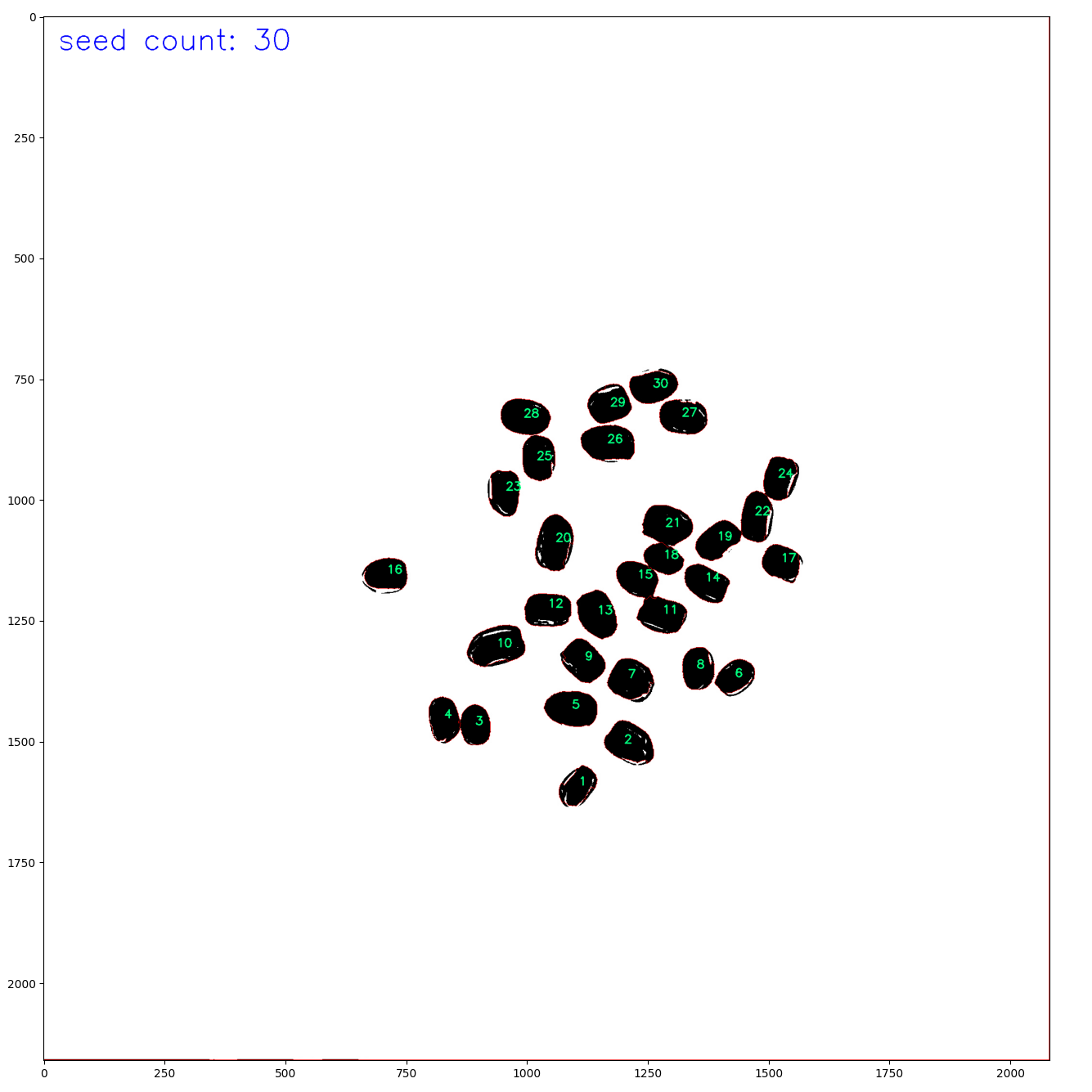 |
📄 전체코드
import numpy as np
import cv2
from matplotlib import pyplot as plt
from typing import Union

class ImageSegmenter:
    def __init__(self, image_path) -> None:
        self.image_path = image_path
        self.img = cv2.imread(self.image_path)
        self.gray = cv2.cvtColor(self.img, cv2.COLOR_BGR2GRAY)
        self.kernel = np.ones((3,3), np.uint8)
        self.font = cv2.FONT_HERSHEY_SIMPLEX
        self.result_image = self.img.copy()  # result_image 속성 추가

    def apply_threshold(self) -> np.ndarray:
        """
        이미지에 임계값을 적용하여 이진 이미지를 생성합니다.

        Returns:
        - thresh: 임계값 적용 후의 이진화된 이미지입니다.
        """
        _, thresh = cv2.threshold(self.gray, 0, 255, cv2.THRESH_BINARY_INV + cv2.THRESH_OTSU)
        return thresh

    def remove_noise(self, thresh: np.ndarray) -> np.ndarray:
        """
        노이즈를 제거합니다.

        Args:
        - thresh: 이진화된 이미지입니다.

        Returns:
        - opening: 노이즈가 제거된 이미지입니다.
        """
        opening = cv2.morphologyEx(thresh, cv2.MORPH_OPEN, self.kernel, iterations = 2)
        return opening

    def get_background_foreground(self, opening) -> Union[np.ndarray, np.ndarray, np.ndarray]:
        """
        배경 및 전경 영역을 확실하게 설정합니다.

        Args:
        - opening: 노이즈가 제거된 이미지입니다.

        Returns:
        - sure_bg: 배경이 확실한 영역입니다.
        - sure_fg: 전경이 확실한 영역입니다.
        - unknown: 배경과 전경을 구분할 수 없는 영역입니다.
        """
        sure_bg = cv2.dilate(opening, self.kernel, iterations=3)
        dist_transform = cv2.distanceTransform(opening, cv2.DIST_L2, 5)
        plt.imshow(dist_transform)
        plt.show()
        _, sure_fg = cv2.threshold(dist_transform, 0.4*dist_transform.max(), 255, 0)
        sure_fg = np.uint8(sure_fg)
        unknown = cv2.subtract(sure_bg, sure_fg)
        return sure_bg, sure_fg, unknown

    def apply_watershed(self, sure_fg: np.ndarray, unknown: np.ndarray) -> np.ndarray:
        """
        워터셰드 알고리즘을 적용합니다.

        Args:
        - sure_fg: 전경이 확실한 영역입니다.
        - unknown: 배경과 전경을 구분할 수 없는 영역입니다.

        Returns:
        - self.img: 워터셰드 알고리즘 적용 후의 이미지입니다.
        """
        _, markers = cv2.connectedComponents(sure_fg)
        markers = markers+1
        markers[unknown==255] = 0
        markers = cv2.watershed(self.img, markers)
        self.img[markers == -1] = [255,0,0]
        return self.img

    def find_contours(self, sure_fg: np.ndarray) -> np.ndarray:
        """
        이진화된 이미지에서 윤곽선을 찾습니다.

        Returns:
        - contours: 찾아진 윤곽선 목록
        """
        contours, _ = cv2.findContours(sure_fg, cv2.RETR_EXTERNAL, cv2.CHAIN_APPROX_SIMPLE)
        return contours

    def binarize(self) -> np.ndarray:
        """
        이미지를 그레이스케일로 변환한 후 이진화를 수행합니다.

        Returns:
        - cv2.bitwise_not(thresh): 이진화된 이미지
        """
        gray = cv2.cvtColor(self.img, cv2.COLOR_BGR2GRAY)
        _, thresh = cv2.threshold(gray, self.threshold, 255, cv2.THRESH_BINARY)
        return cv2.bitwise_not(thresh)

    def annotate_contours(self, image: np.uint8, contours: np.ndarray) -> np.ndarray:
        """
        윤곽선을 이미지에 그리고, 각 윤곽선의 중심에 번호를 부여합니다.

        Args:
        - image: 윤곽선을 그릴 이미지
        - contours: 윤곽선 목록

        Returns:
        - image: 윤곽선과 번호가 추가된 이미지
        """
        for i, contour in enumerate(contours):
            M = cv2.moments(contour)
            if M["m00"] != 0:
                cX = int(M["m10"] / M["m00"])
                cY = int(M["m01"] / M["m00"])
                cv2.putText(image, str(i + 1), (cX, cY), cv2.FONT_HERSHEY_SIMPLEX, 0.8, (0, 255, 127), 2)
        return image

if __name__ == "__main__":
    image_path = 'SEED_COUNTER\seed_count_image.jpg'
    IS = ImageSegmenter(image_path)
    thresh = IS.apply_threshold()
    opening = IS.remove_noise(thresh)
    sure_bg, sure_fg, unknown = IS.get_background_foreground(opening)

    image = IS.apply_watershed(sure_fg, unknown)
    contours = IS.find_contours(sure_fg)
    cv2.putText(image, f"seed count: {len(contours)}", (30, 70), IS.font, 2, (0, 0, 255), 2)
    annotated_image = IS.annotate_contours(image, contours)  # 수정된 메소드 호출
    plt.imshow(annotated_image)
    plt.show()