NA-linear_equation1
1. Introductions
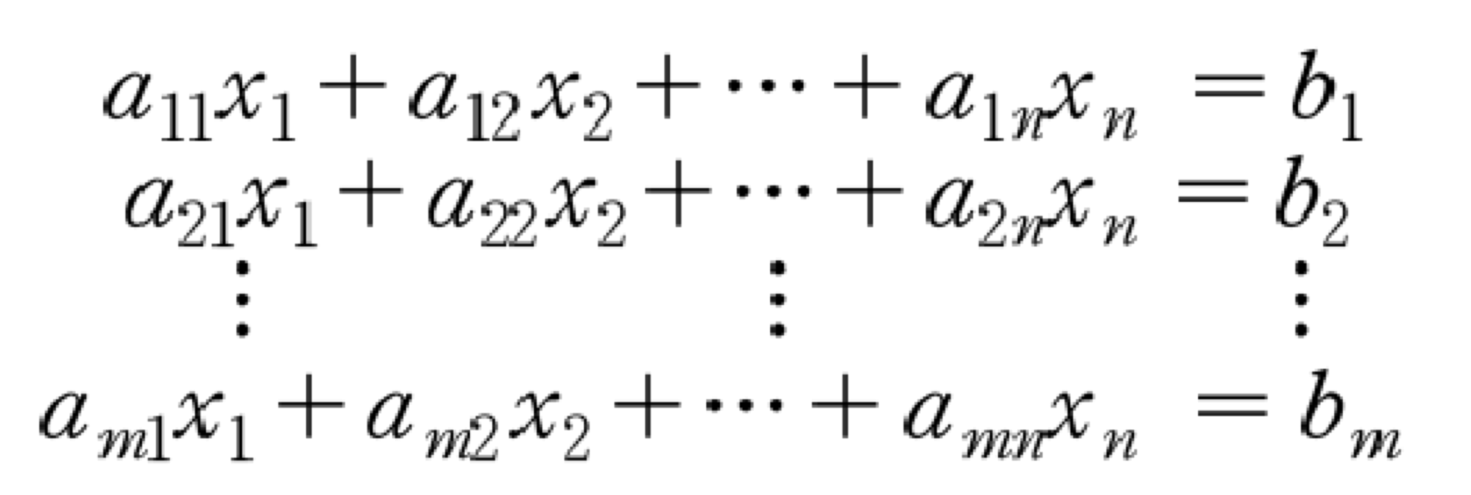
1) Linear equations
- N unknowns, M equations
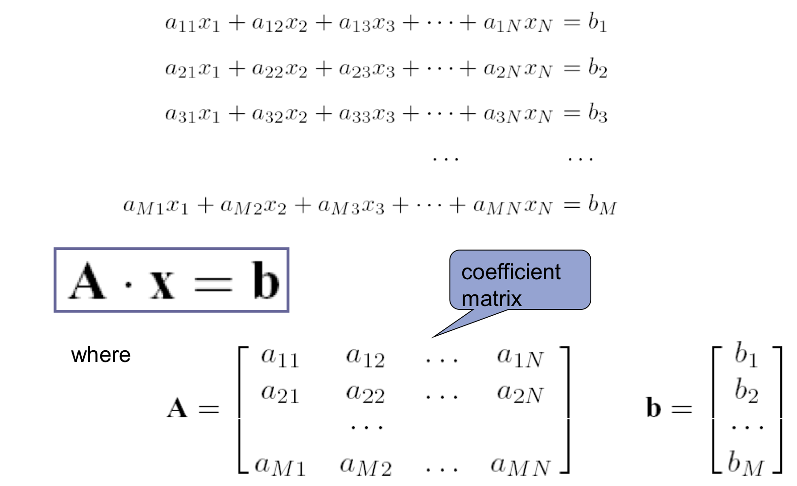
- equation의 개수가 적으면, 답이 많을 수 밖에 없다.
2) Approach
- Direct methods
- Gauss elimination
- Gauss-Jordan elimination
- LU decomposition
- (Singular value decomposition)
- Iterative methods
- Jocobi iteration
- Gauss-Seidel iteration
3) Basic properties of matrices
a) Basic matrices
- square matrix (N=M)
- Row Matrix (하나의 Row만을 가지는 것,)
- Column Matrix (하나의 Column만을 가지는 것)
- diagonal matrix (diagonal 성분만 가지고 있는 것)
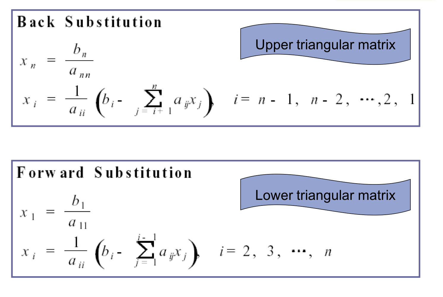
- upper/lower triangular matrix (윗, 아랫 부분만 0이 아닌 것)
- tri-diagonal matrix (diagonal과 그 아래 위 성분들이 0이 아닌 것)
- transposed matrix: A^t
- symmetric matrix: A = A^t
- orthogonal matrix: A^tA = I 즉, A^-1 = A^t
b) Basic properties
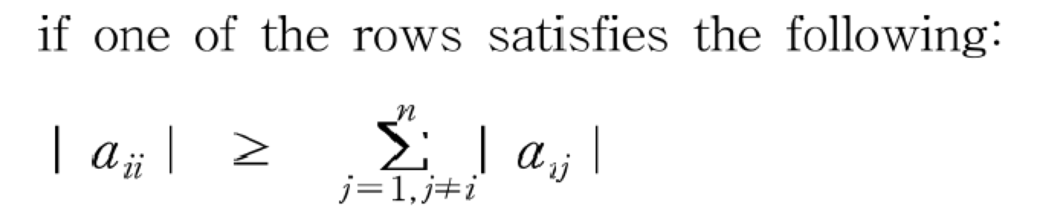
- Diagonal dominance (즉, diagonal 성분이 다른 성분들 보다 큰 것)
- Transpose facts
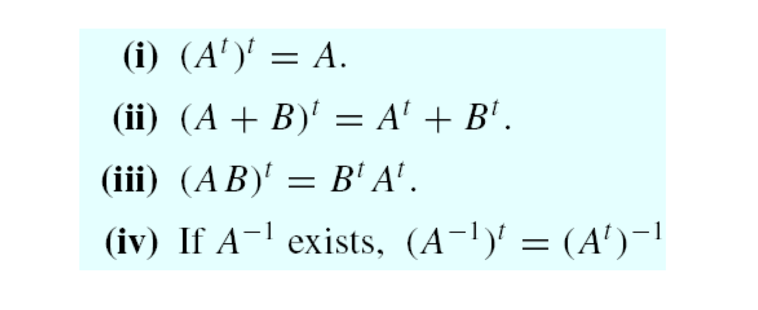
- |A| = det(A) (외적 계산하는 방식임)
c) Determinant facts
-
Product Theorem:
det(AB) = det(A)det(B)
-
If A is upper(or lower) diagonal,
det(A) = diagonal 성분들의 곱이다.
-
det(A^t) = det(A)
-
A의 두 열을 교환할 때 마다 determinant의 부호가 바뀐다.
det(B) = -det(A)
-
어떤 scalar s에 대해서,
det(sA) = s^n*det(A)
det(-A) = (-1)^n*det(A)
-
만약 rowi(A) = c*rowj(A), (j ≠ i, c is a constant) 이라면, det(A) = 0이다.
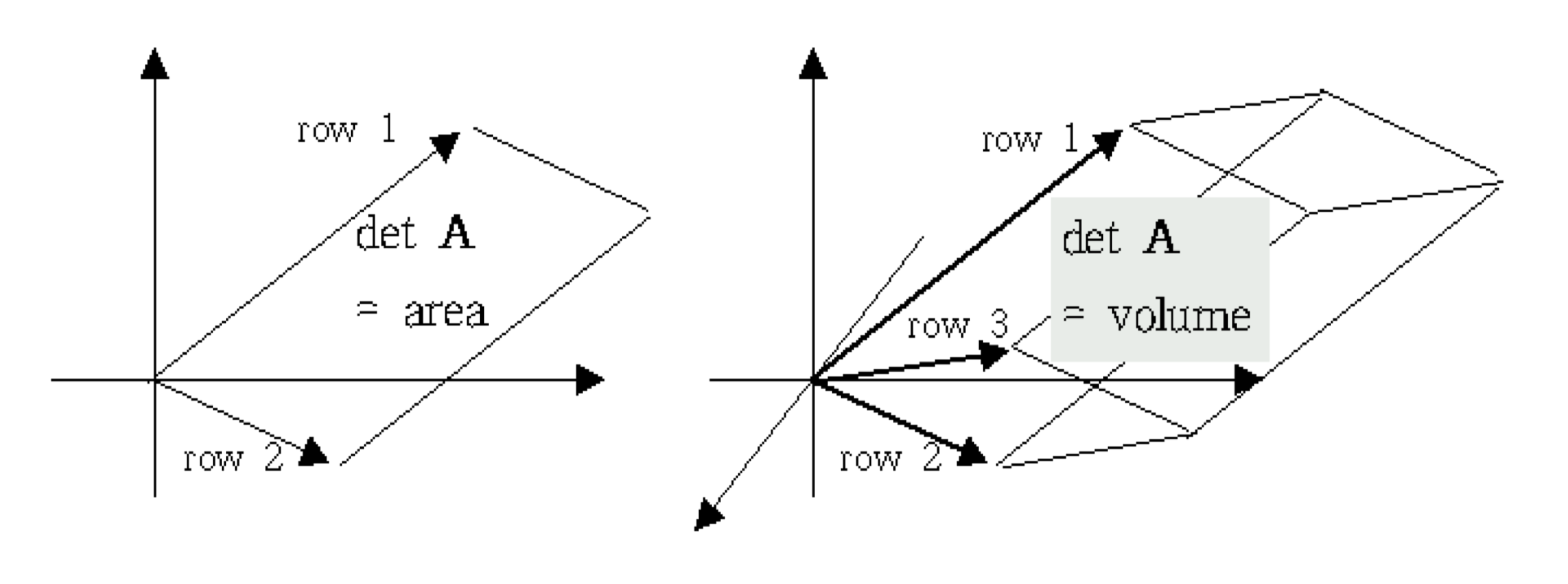
d) Geometrical interpretation of determinant
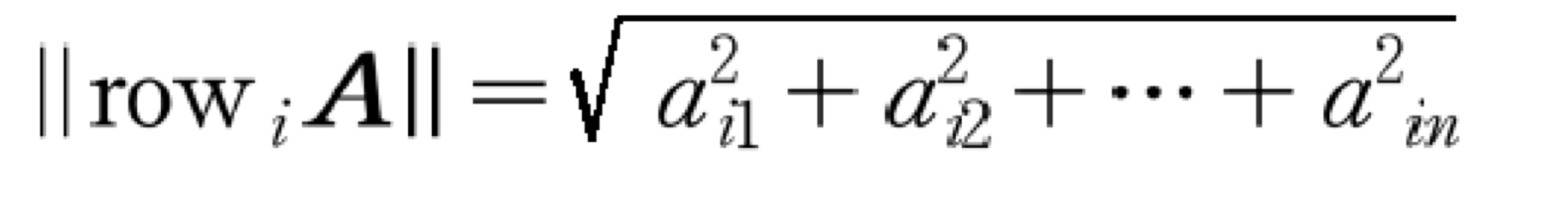
- Euclidean length
- Volumn
- Hadamard’s inequality (모든 row 성분이 직교 해야 최댓값을 갖기 때문이다.)
|detA| ≤ ||row1A|| ||row2A|| … ||rownA||
4) Over-determined / Under-determined problem
- Over-determined problem (m>n)
- 제한이 너무 많다. 조건이 많을 수록 구하기가 힘들다.
- least-square estimation
- 데이터와 모델간의 차이의 제곱 합을 최소화하는 해를 찾는다.
- robust estimation etc.
- 이상치의 영향을 최소화하여, 확실히 이상한 값은 버린다.
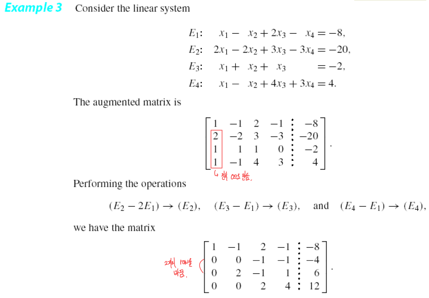
5) Augmented matrix
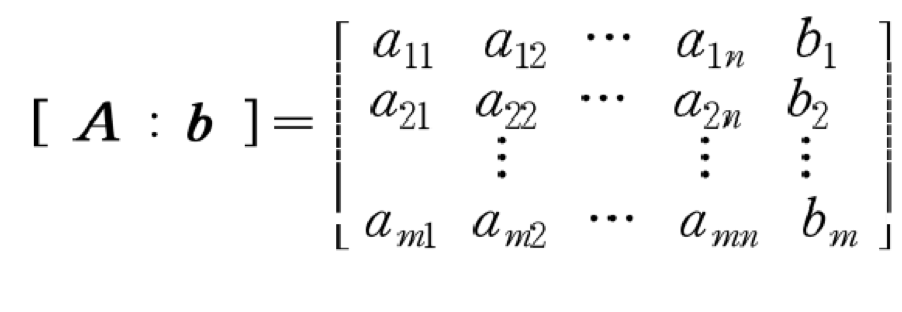
- Elementary row operations
- 행 연산을 수행 할때, 연립방정식의 해에 영향을 주지는 않는다.
- multiply a constant( ≠ 0 ) to i-th row
- change the order of rows
- constant를 곱한 행을 다른 행에 더하는 것.
6) Cramer’s rule
- 만약 det(A) ≠ 0이라면, soultaion Ax = b는 다음과 같다.
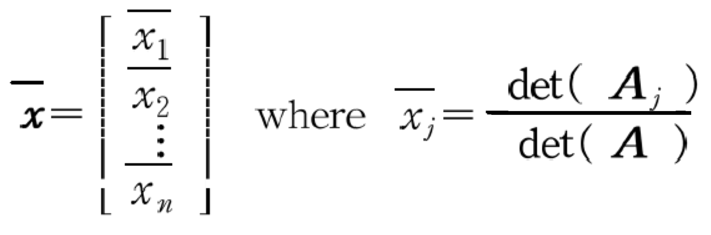
이때, Aj matrix는 A matrix에서 j 번째 column이 b로 바뀐 matrix이다.
- det(A) = 0인 것의 의미
- det(A)가 0인 행렬은 역행렬이 존재하지 않는다.
- 연립 방정식의 해가 없거나 무한한 수의 해를 가질 수 있다.
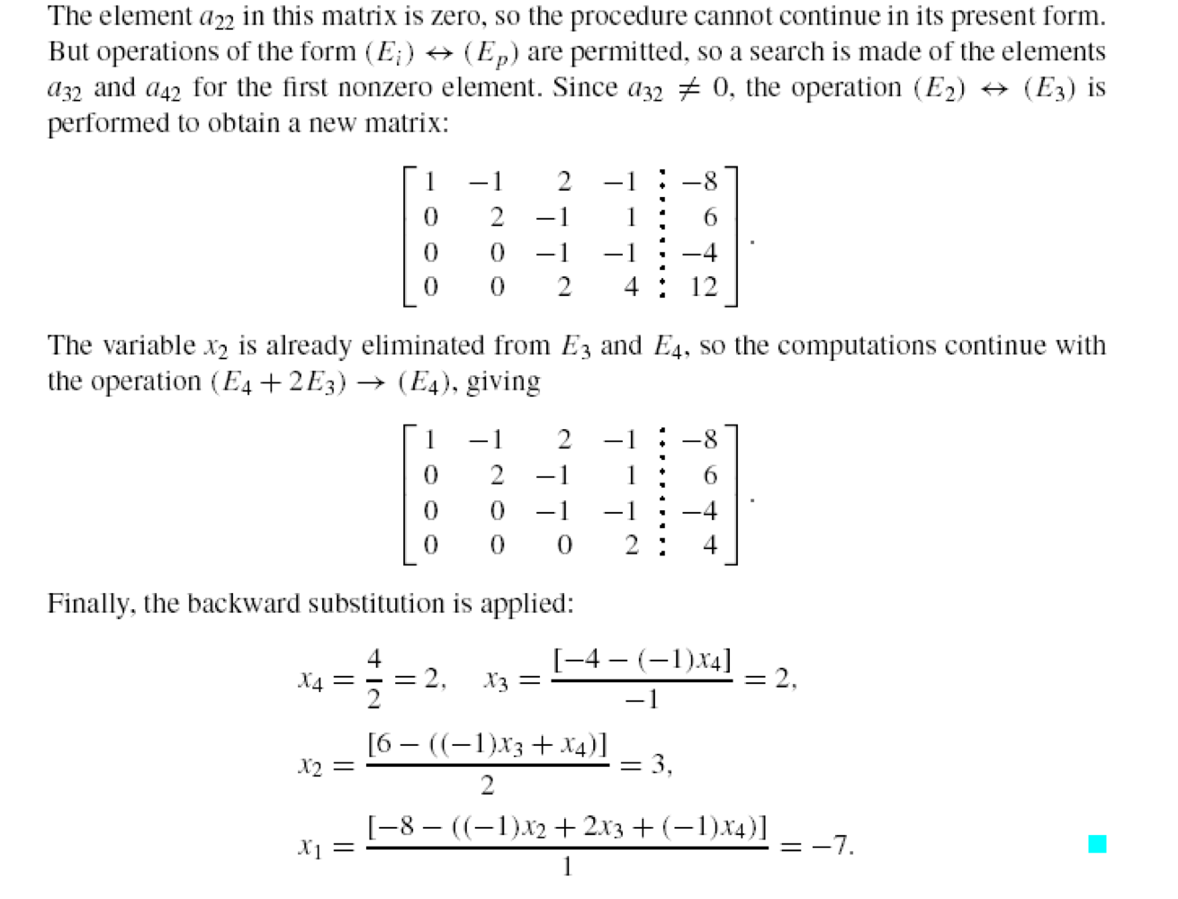
7) Triangular coefficient matrix
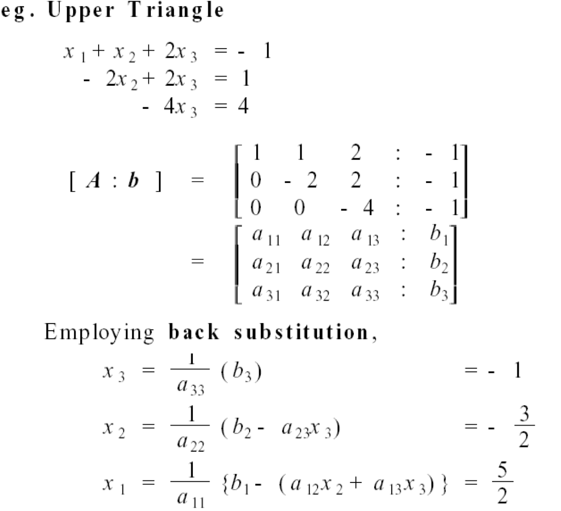
- x3부터 대입만 해도 쉽게 값을 구할 수 있다.
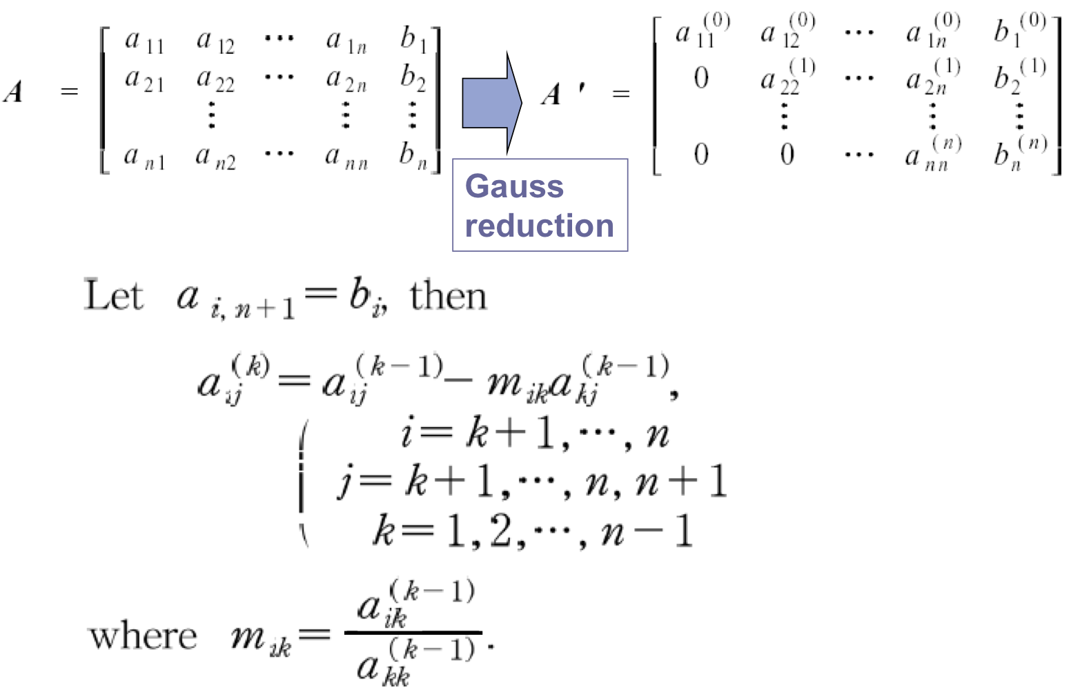
2. Gauss elimination
- Step 1: Gauss reduction
- = Forward elimination
- Coefficient matrix → upper triangular matrix
- Step 2: Backward substitution
a) Gauss reduction
- upper triangular matrix로 만드는 과정이다.
b) Troubles in Gauss elimination
- pivot coefficient에서 round-off error의 부정적인 여향이 있을 수 있다.
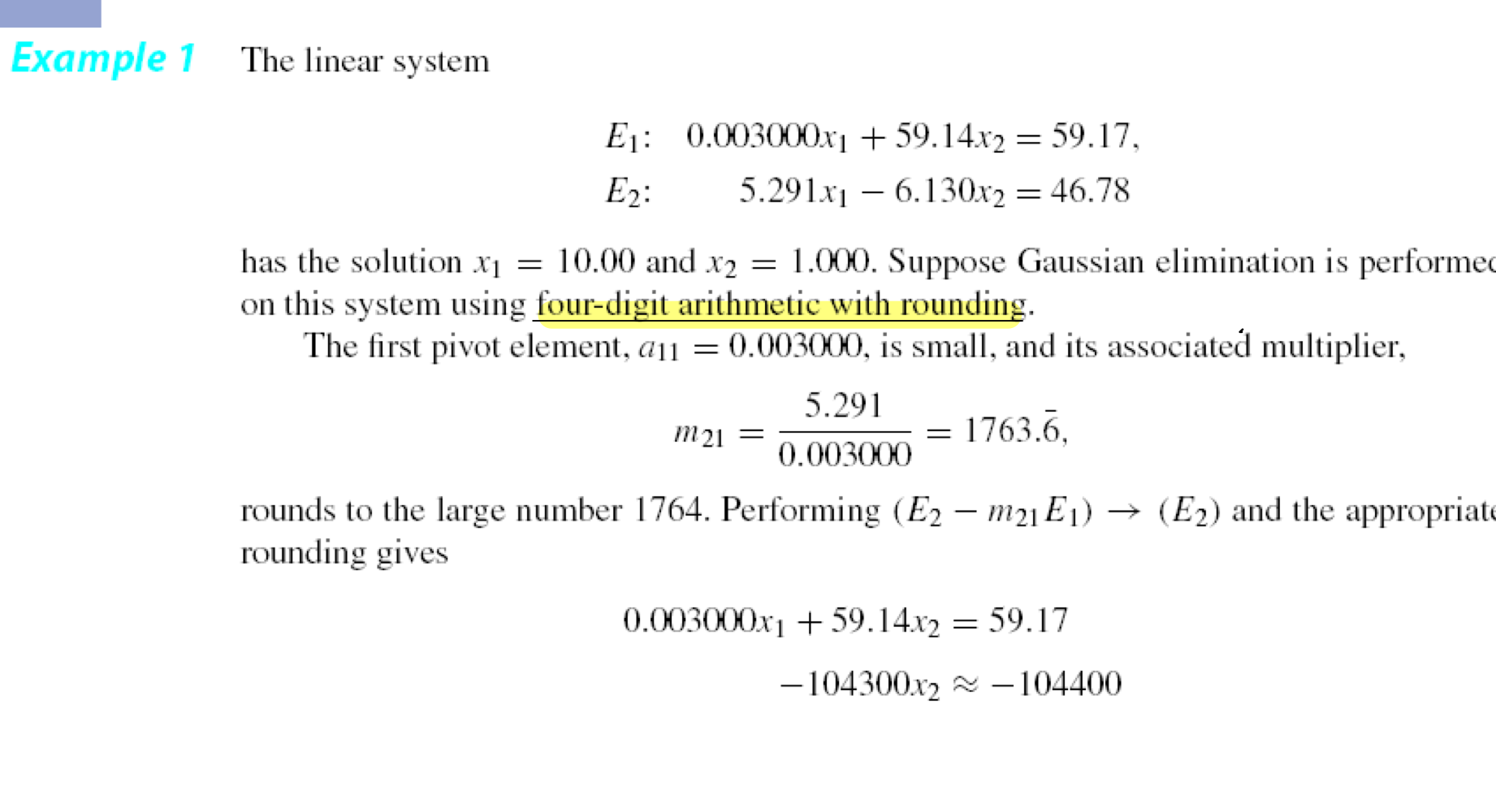
- 소수점 4자리까지만 표현 할 수 있기에, 어쩔 수 없이 버려지는 값이 생긴다.
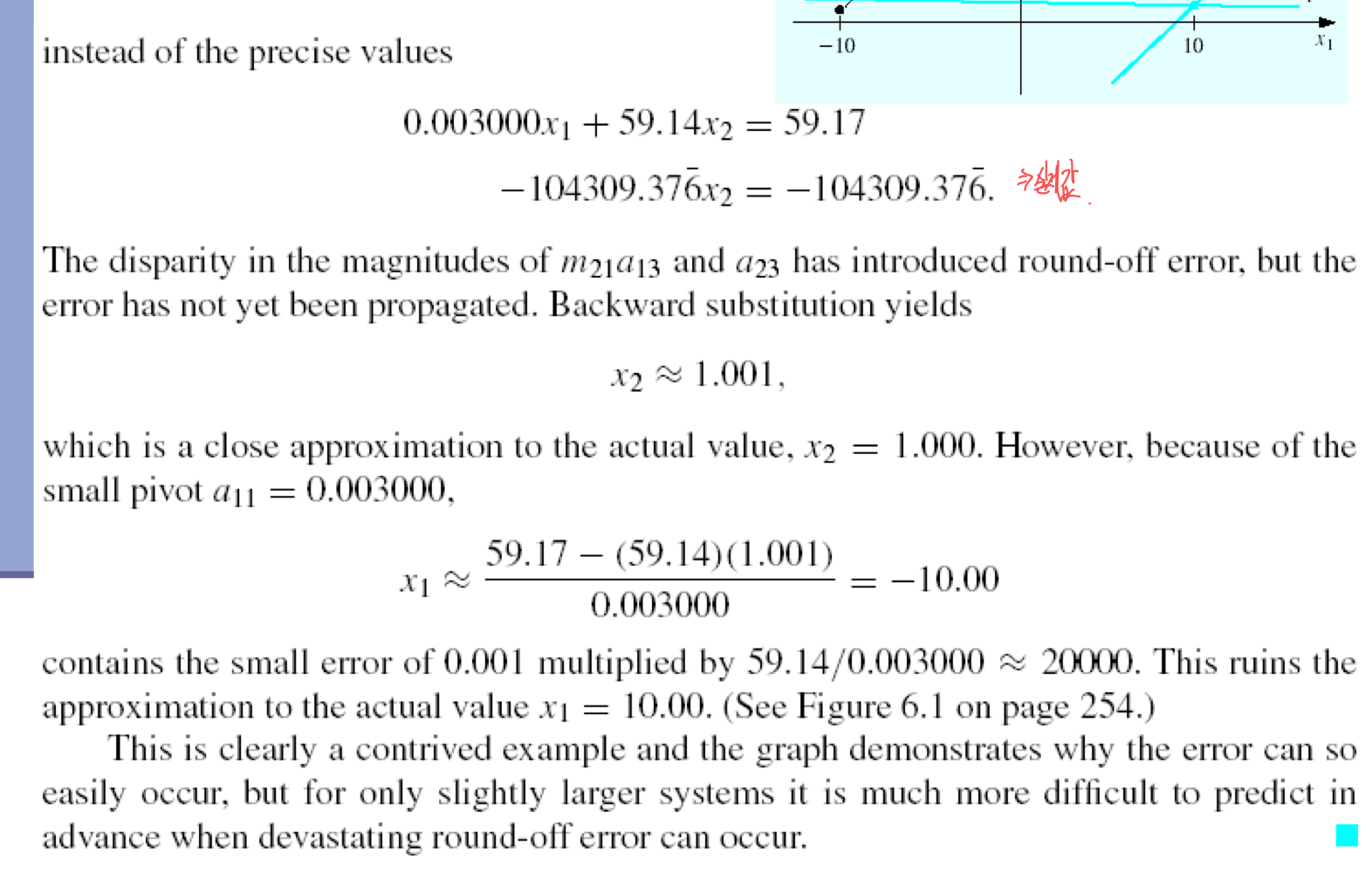
- 조그만 차이이지만, x1의 값이 많은 차이가 발생한다.
c) Pivoting strategy
- 즉, 가장 큰 값을 처리하고자 하는 위치에 놓는 방식이다.
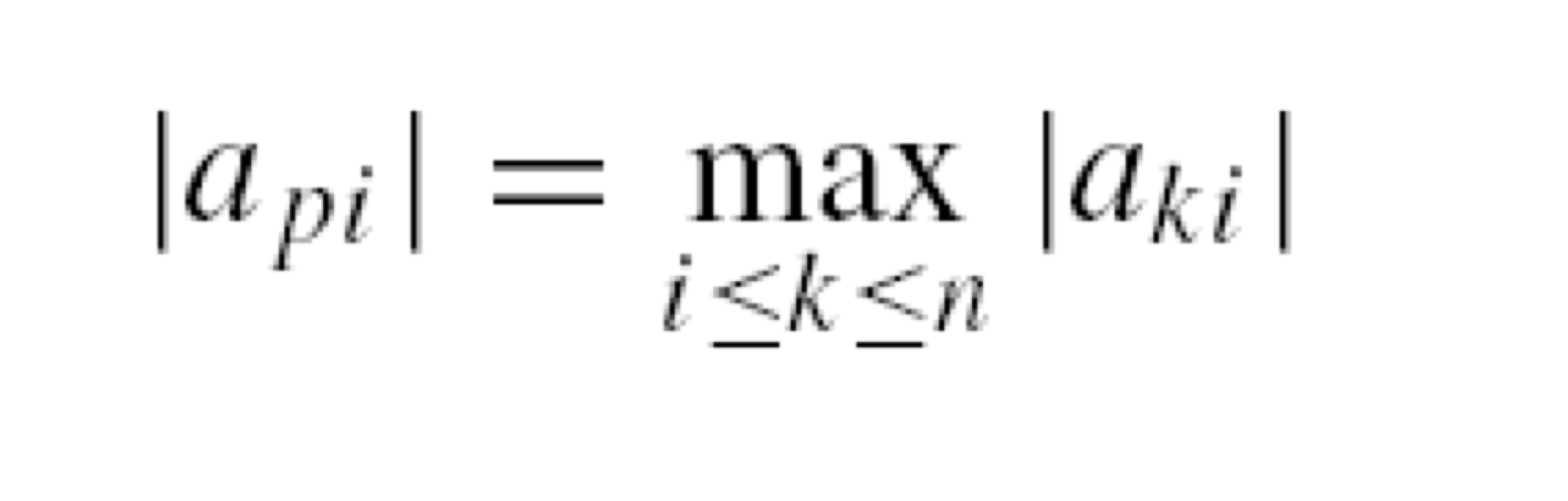
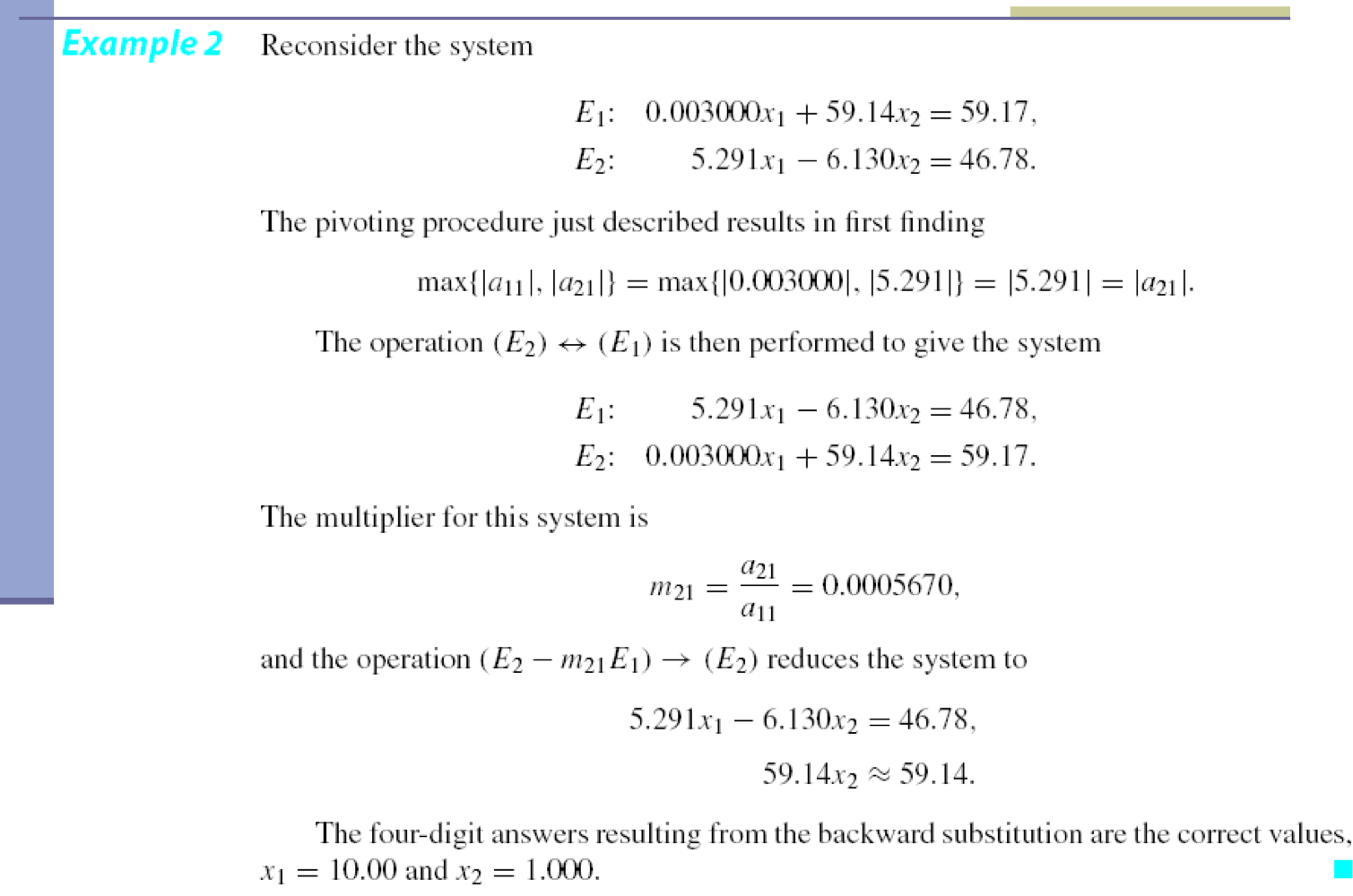
- a11과 a21을 비교하여 더 큰 값을 위로 올려서 계산한다.
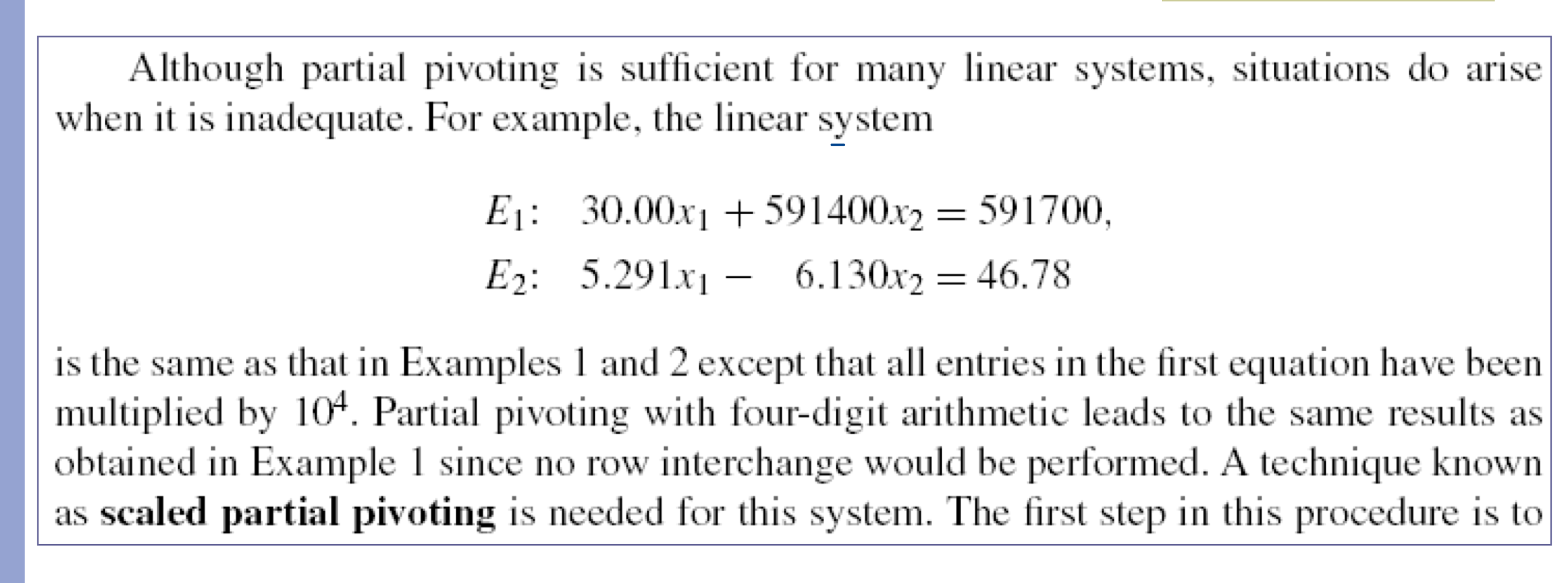
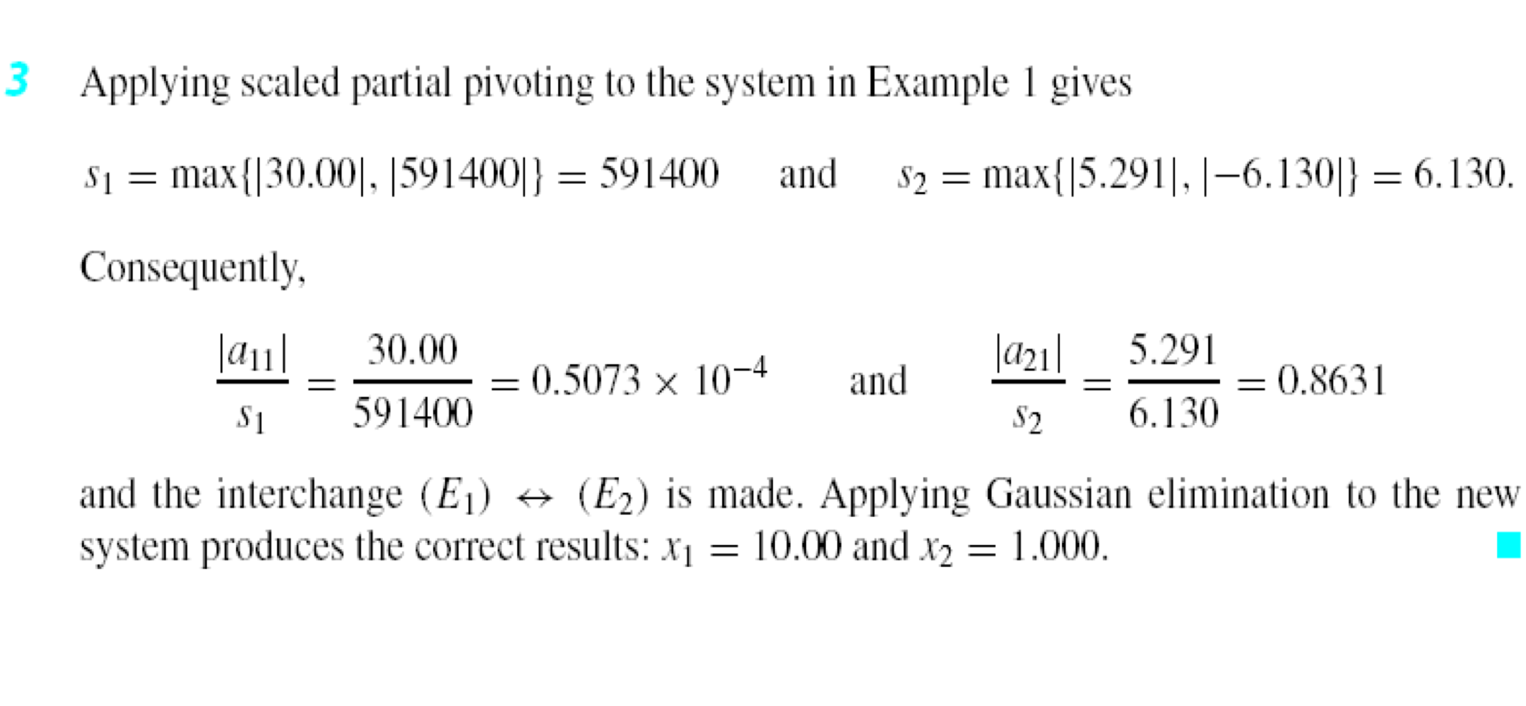
d) Scaled partial pivoting
- 각 행 좌변 요소 중 가장 큰 값을 통해 normalize 한 후 pivoting을 진행하는 방식이다.
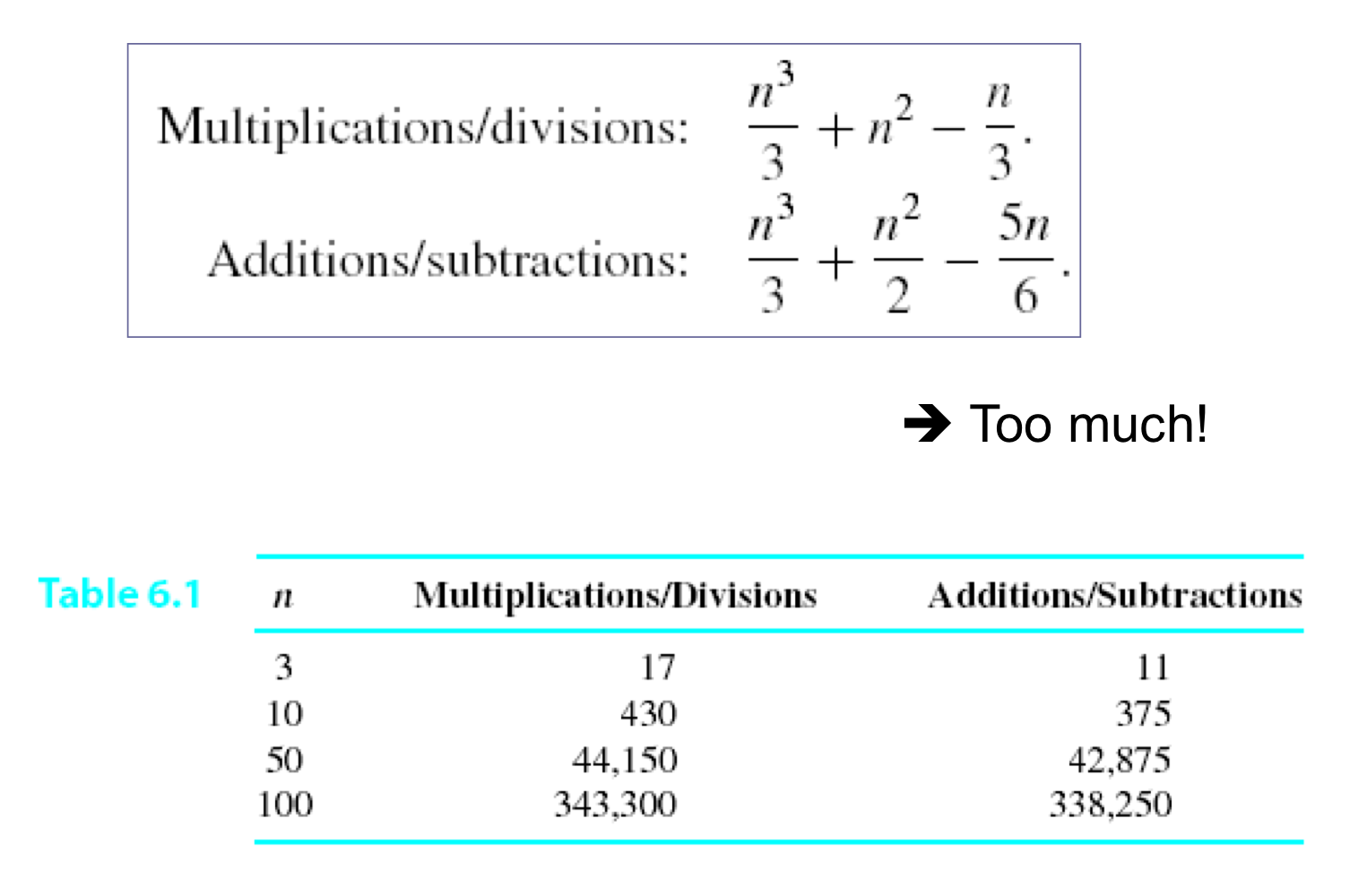
e) Complexity of Gauss elimination
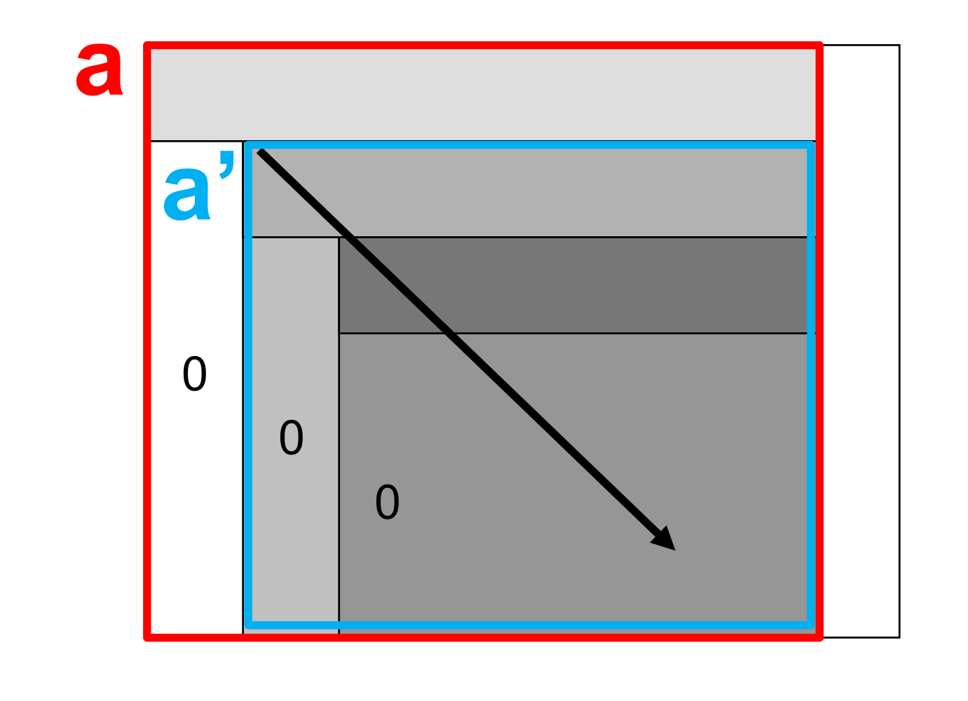
f) Summary: Gauss elimination
- Normalization: 모든 row를 normalize한다.
- Partial pivoting: 가장 큰 값을 uppermost에 둔다.
- 행들의 1번째 요소를 0으로 만든다.
- a의 submatrix a’에 대해서 위의 과정을 반복한다.
- backward substitution을 통해 값을 얻는다.
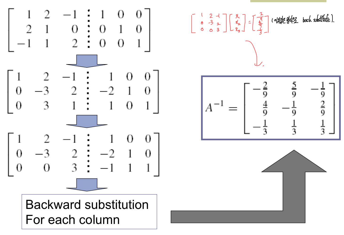
3. Gauss-Jordan elimination
- off-diagonal 요소들이 모두 0이 될때 까지 없앤다.
- Gauss elimination보다, 50%의 계산이 더 소요된다.
- inverse matrix를 얻는 좋은 방법이다.
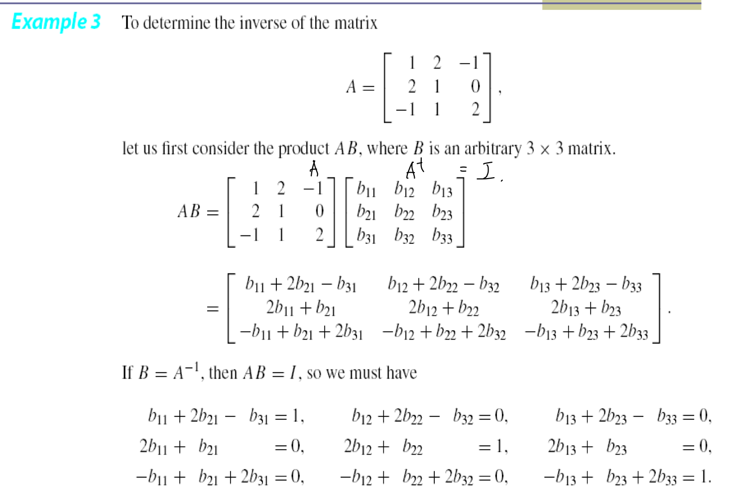
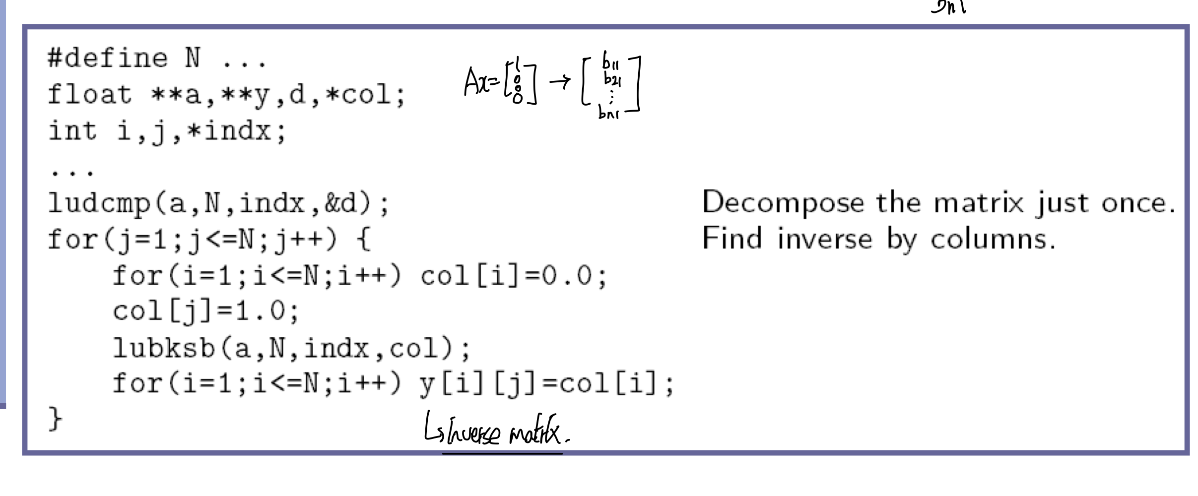
1) Obtaining inverse matrix
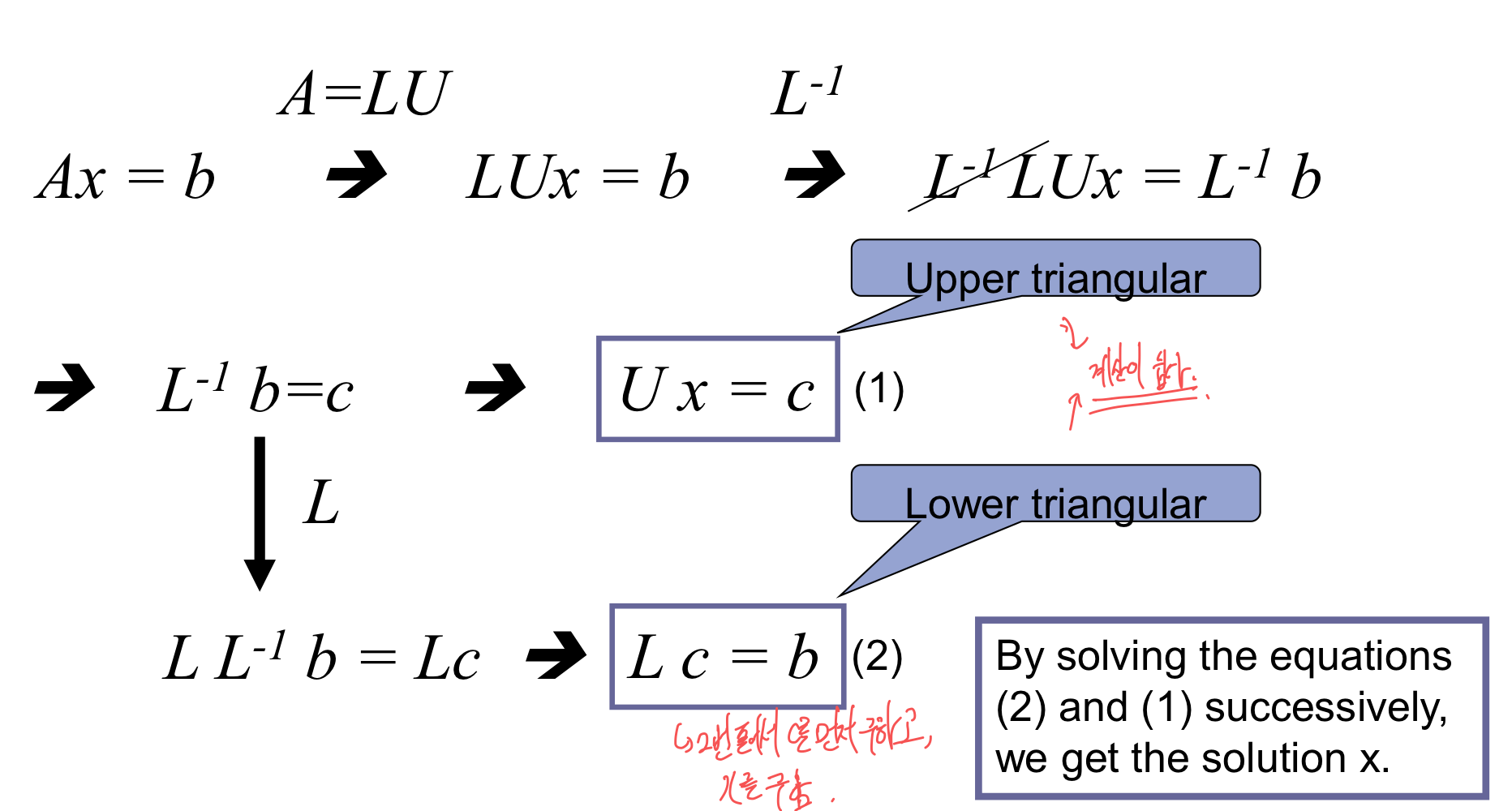
4. LU decomposition
- 원리: lower triangular matrix와 upper triangular matrix로 decomposite를 하여, 값을 구하는 방식이다.
1) Various LU decompositions
- Doolittle decomposition
- Lij = 1, for all i
- Crout decomposition
- Uii = 1, for all i
- Cholesky decomposition
- Lii = Uii
- symmetric, positive-definite matrix에 적절하다.
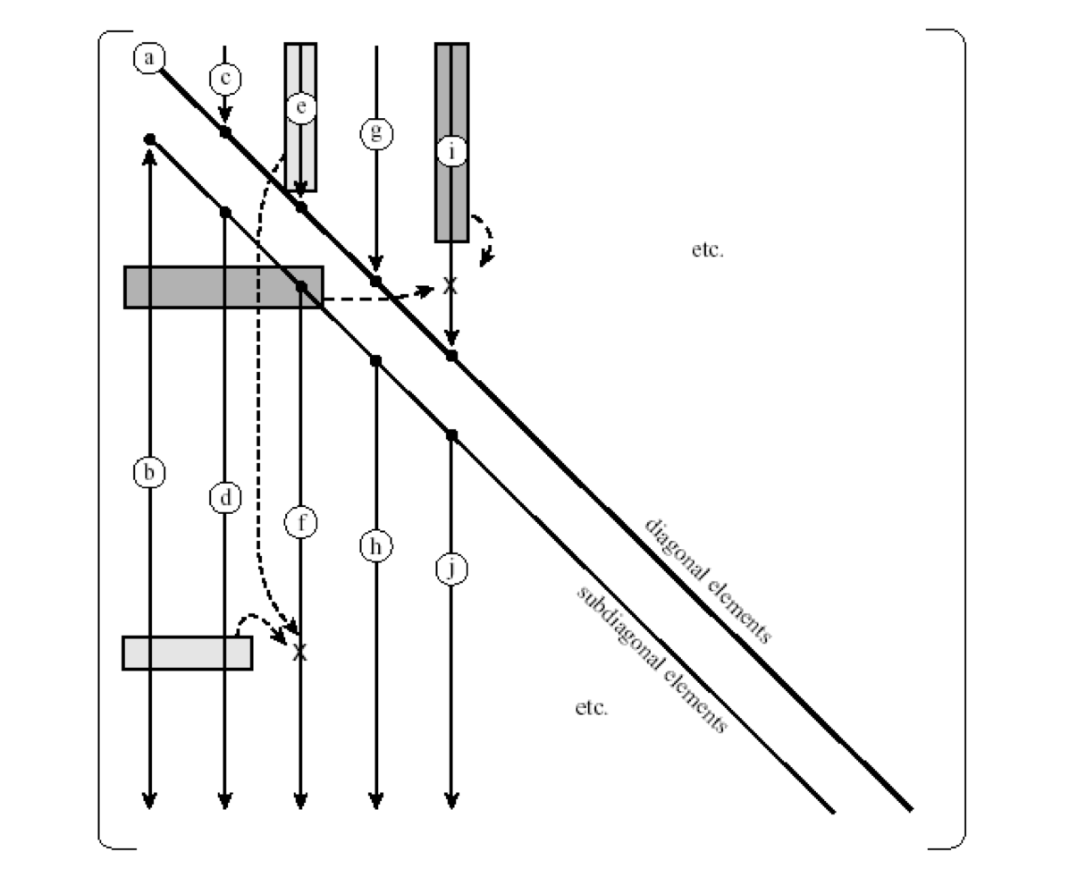
2) Crout decomposition
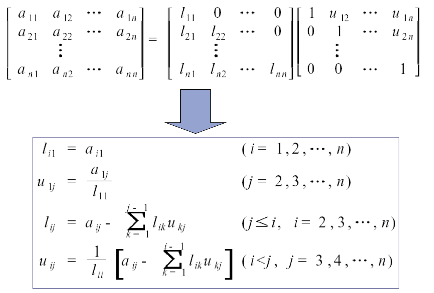
- LU matrix를 각각 메모리를 나누어 쓰면 비효율적이기에, 1개의 matrix에 LU를 모두 넣는다.
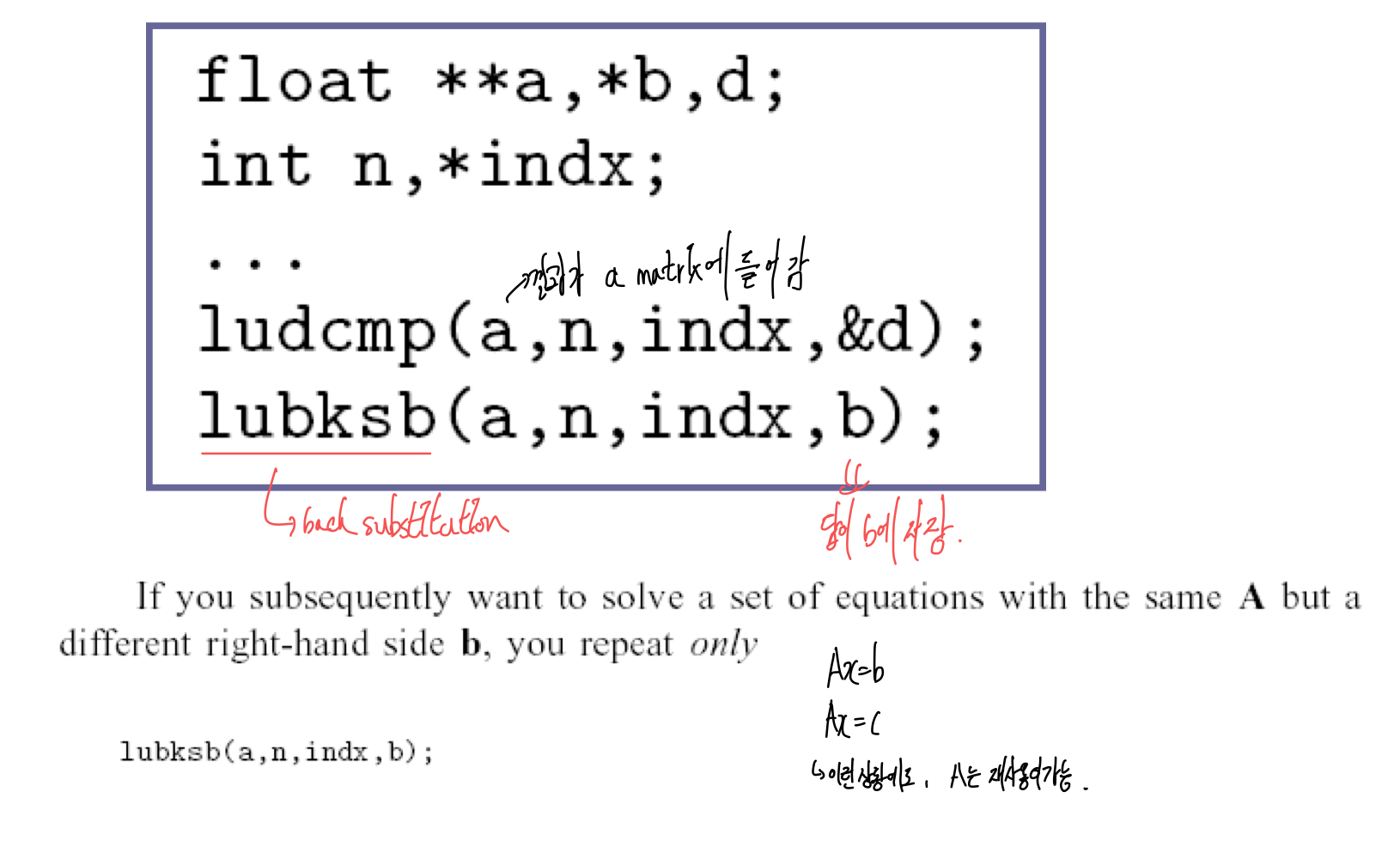
3) Programming using NR in C
- linear equations의 set을 구하는 것
- Obtaining inverse matrix
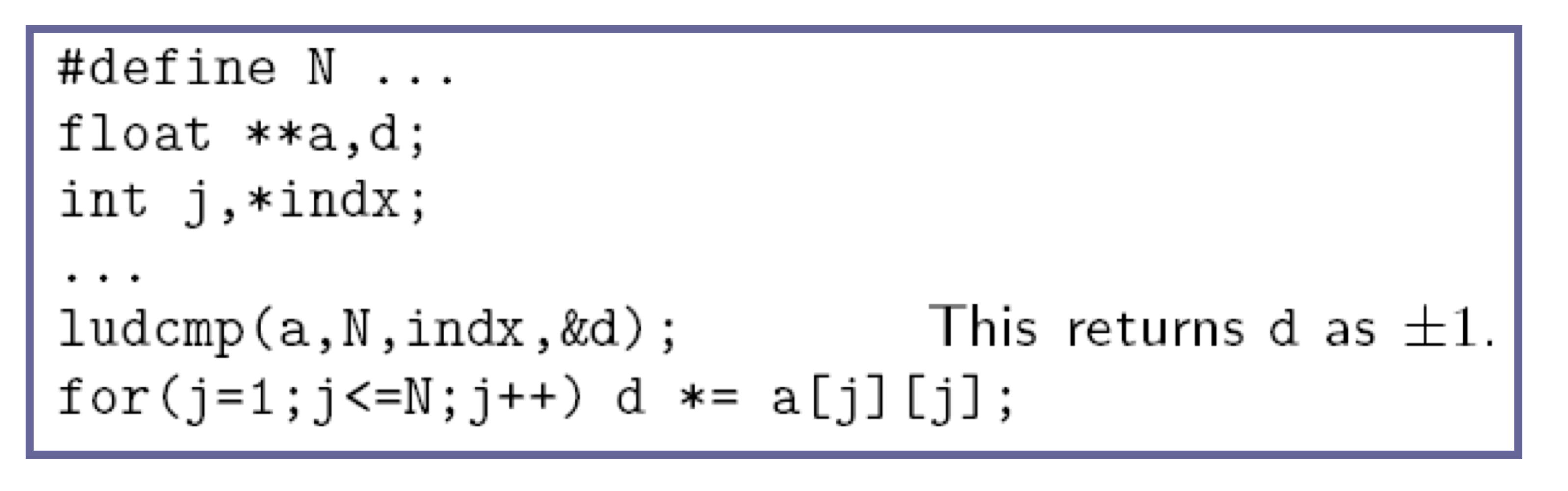
- Calculating the determinant of a matrix
4) Iterative Improvement of a Solution
- Iterative improvement
- 정확한 값 x
- contaminated solution x’ = x + dx
- wrong product b’ = b + db
- Algorithm derivation A(x+dx) = b + db Since Ax = b Adx = db Solving the equationg to get the improvement dx = A^-1db 즉, 해당 dx값을 가지고 계속해서 반복한다. (A는 고정시키고 db만 바꾸면 이것이 가능하다.)
- Numerical aspect
- Using LU decomposition
- 일단 한번 decomposition을 하면, db를 사용해서 substitution을 한다면, dx를 계속해서 보정 할 수있다.
- mprove() in NR in C
- Using LU decomposition
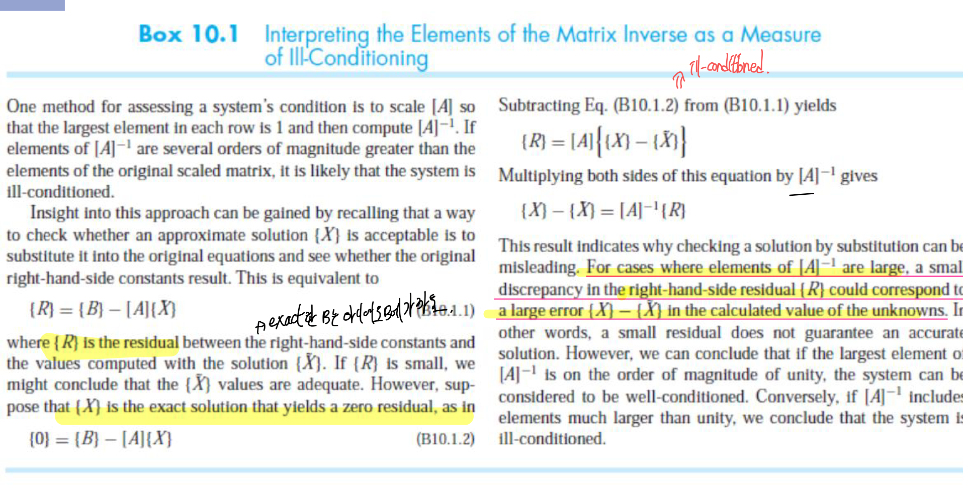
- Measure of ill-conditioning
- A’: normalized matrix
- If A’^-1 is large → ill -conditioned