1. Singular Value Decomposition(SVD)

1) Why SVD?

• Gaussian Elim. and LU Decomposition은 singular나 singular에 근접한 matrix에 대해서 만족할만한 결과를 주지 못한다.
• SVD는 over- or under determined problems를 해결 할 수 있다.
• SVD는 orthonormal basis vector를 만든다.

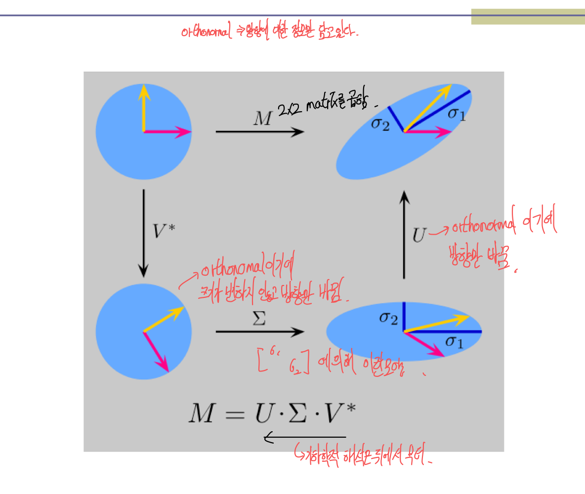
2) What is SVD?

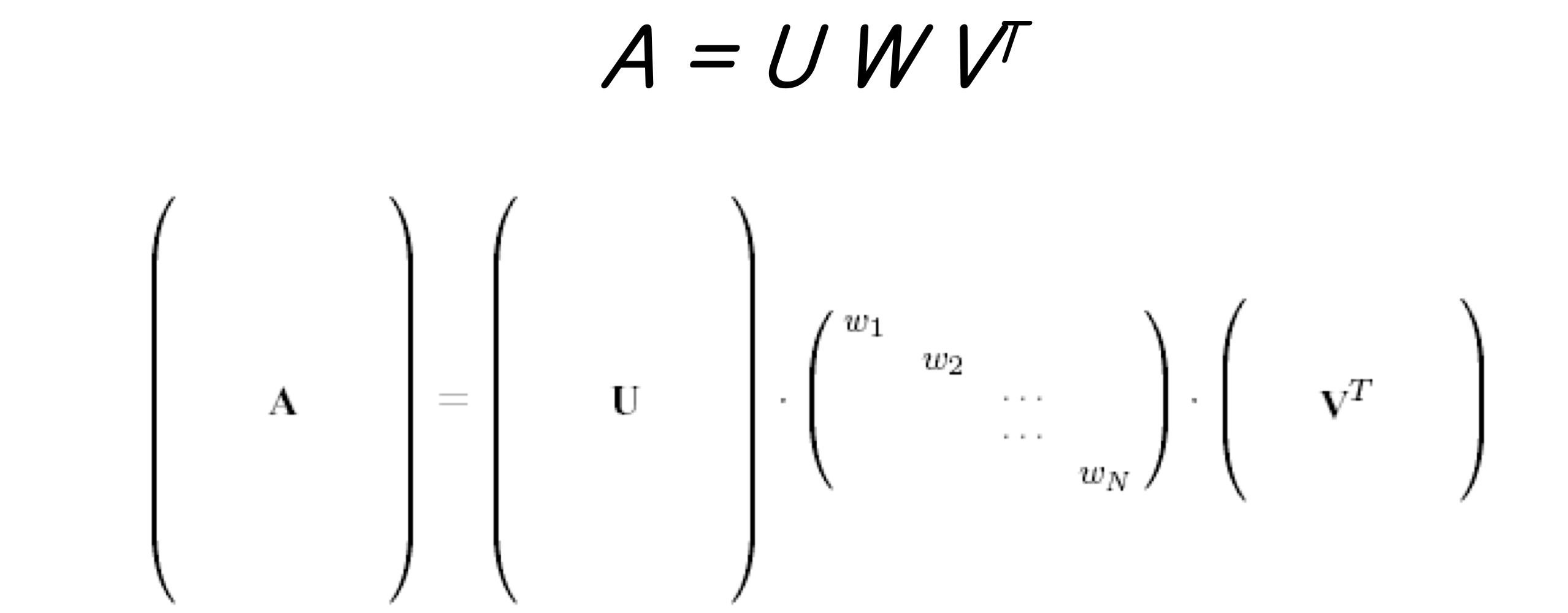
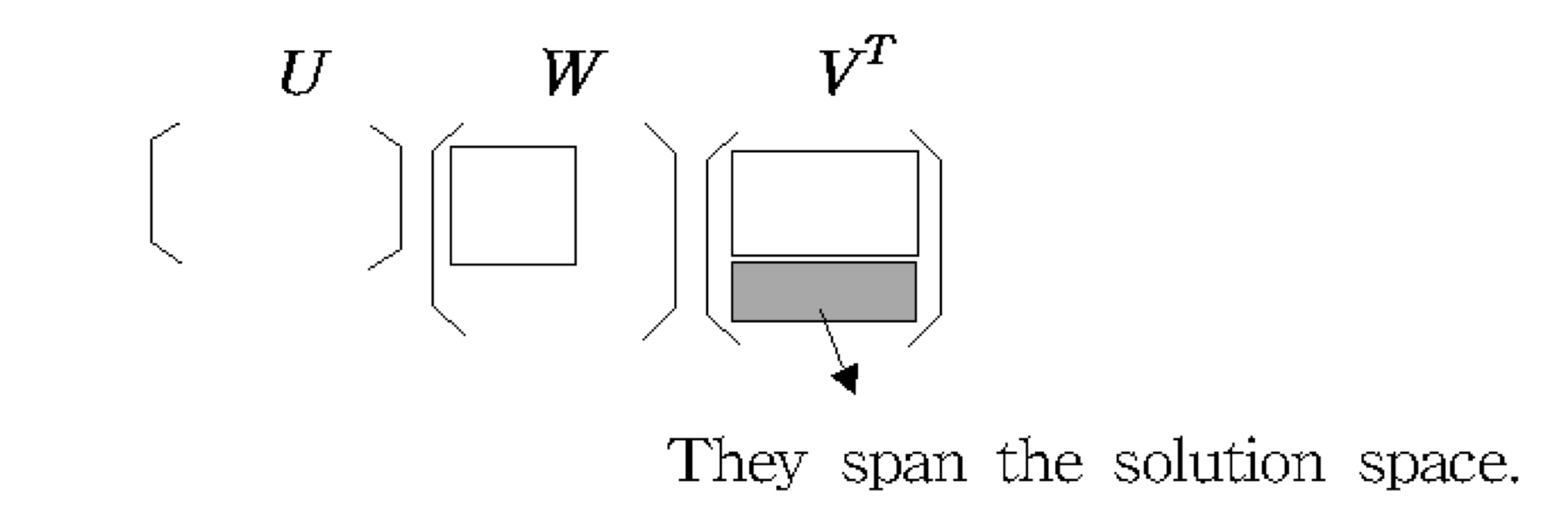
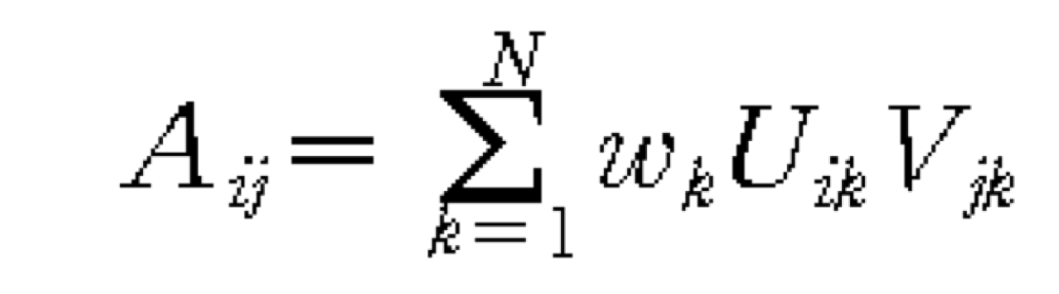
• 어떤 MxN matrix A에 대해서도, MxM matrix U, MxN matrix W, NxN matrix V^T로 decomposition 할 수 있다.
• U와 V matrix는 크기가 1이고, orthogonal 하다 (orthonormal matirx)
• 앞 뒤 matrix의 크기가 1이니까, 크기는 W에 모두 몰리게 된다. (w 성분 중 0이 있으면 N차원이 만족하지 않는다.)

a) Properties of SVD

• Orthonormality
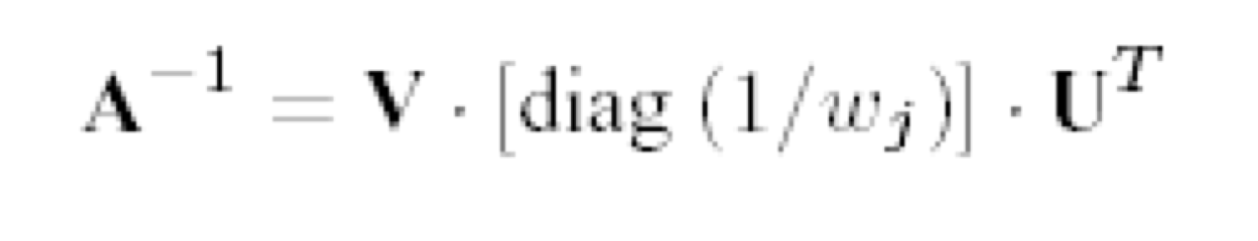
  • U^TU = I ⇒ U^-1 = U^T
  • V^TV = I ⇒ V^-1 = V^T
• Uniqueness
  • decomposition은 singular matrix이든 아니든 항상 가능 하며, 거의 유일하다.

b) SVD of a square matrix

• SVD of a square matrix

• Columns of U
  • an orthonormal set of basis vectors
• wj’s의 성분이 0인 것에 상응하는 V의 column
  • an orthonormal basis for the nullspace

c) Interpretation of SVD

3) Reminding basic concept in linear algebra

• Important Concept in Ax=b of order N
  • Range: {y | y = Ax } (subspace of b that can be reached by A)
  • Rank: dimension of Range
  • Nullspace: {x | Ax = 0 }
  • Nullity: dimension of Nullspace
  • N = rank + nullity

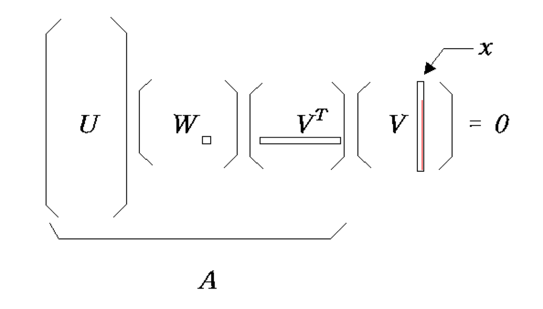
4) Homogeneous equation

• Homogeneous equations (b =0 ) + A is singular
  • wj가 0인 것에 상응하는 V column은 solution을 만든다. (solution space를 형성한다.)

5) Nonhomogeneous equation

• Nonhomogeneous eq. with singular A

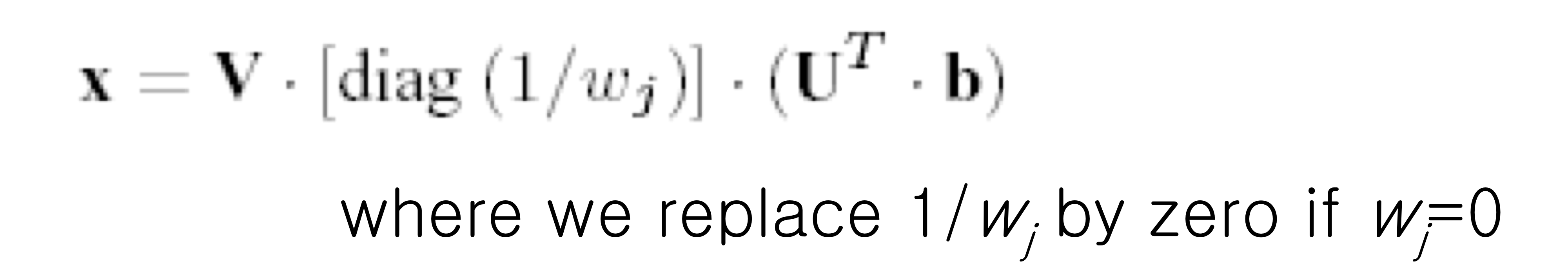
• singular라면 답이 겁나 많은 거기에 wj = 0으로 두어서 답을 하나로 고정시킨다.
• 또한, 이렇게 SVD의 solution을 정한다면, solution vector는 항상 가장 짧은 길이를 가진다.
• 만약, b가 A의 range에 들어있지 않다면,
  • x 는 r = |Ax -b|가 최소가 되는 값을 가진다. (least-square sense)

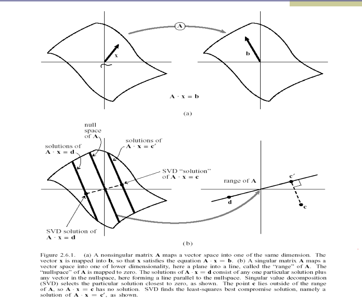
• 만약, nullity가 0이라면(rank가 full rank) → x는 b로가는 유일한 답을 가진다.
• 만약, nullity가 0이 아니라면(평면에서 직선)
  • SVD solution이 A의 range안에 있다면 → answer (원점에서 가장 가까운 점)
  • SVD solution이 A의 range안에 없다면 → least-square sense (range에서 가장 가까운 점을 answer로 택한다.)

6) SVD - under/over-determined problems

• SVD for Fewer Equations than Unknowns

• SVD for More Equations than Unknowns
  • SVD는 least-square solution을 만든다.
  • 일반적으로 singular하지 않음

7) Application of SVD

• Applications
  • Constructing an orthonormal basis
    • M-dimensional vector space
    • Problem: Given N vectors, find an orthonormal basis
    • Solution: U matrix의 Columns들이 orthonormal basis이다.
  • Approximation of Matrices

• w성분중에 가장 큰 것만 보고 뒤에꺼를 무시해도 어느정도의 data를 파악 할 수 있다. (PCA)

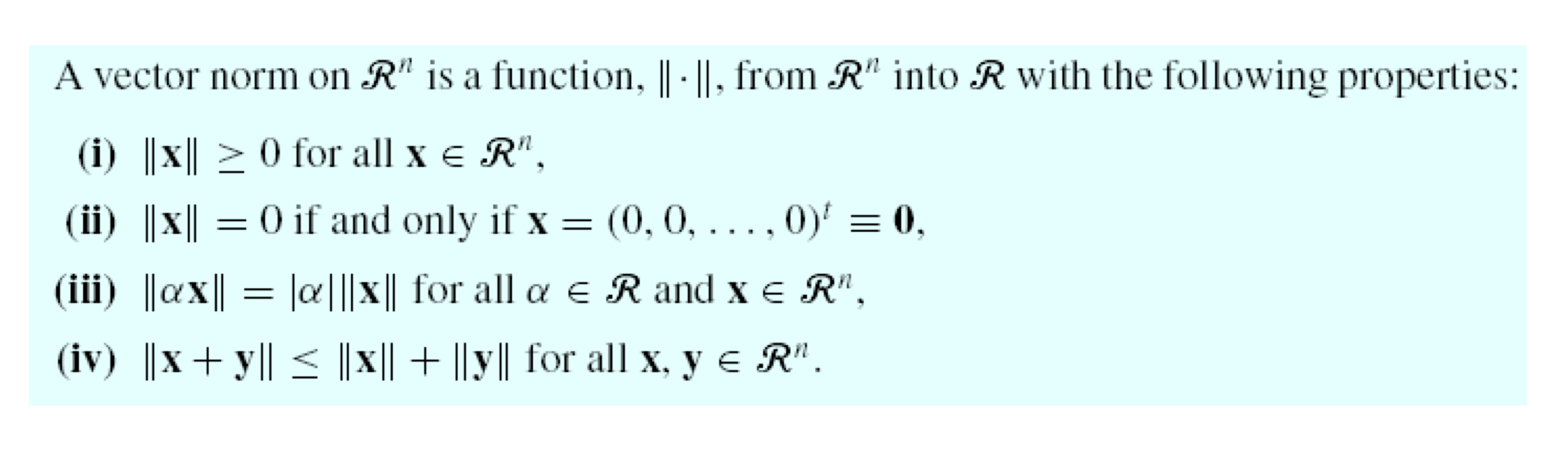
2. Vector Norm

1) Introductions

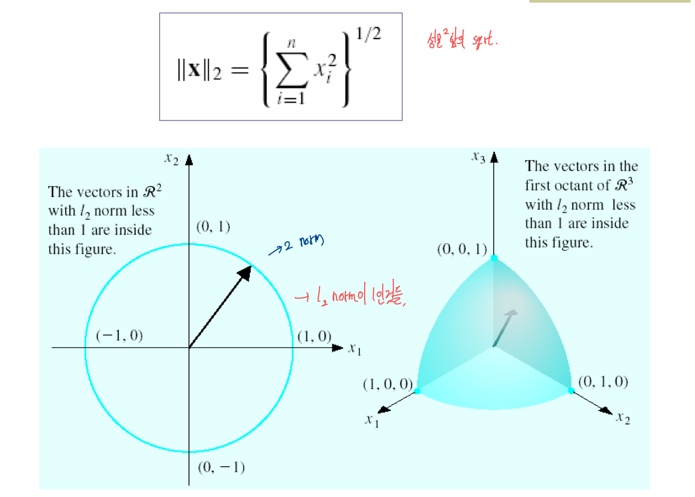
2) I2 norm

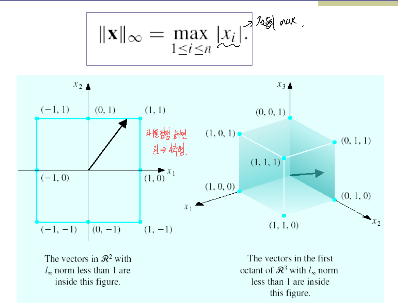
3) I∞ norm

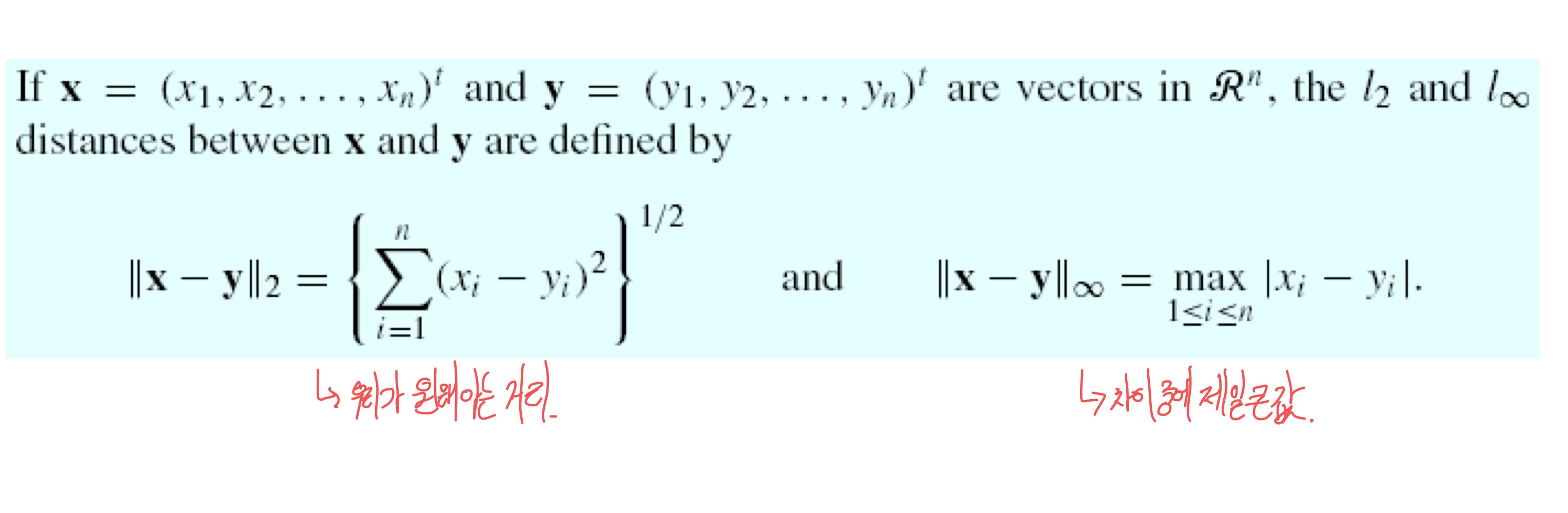
4) Distance between vectors

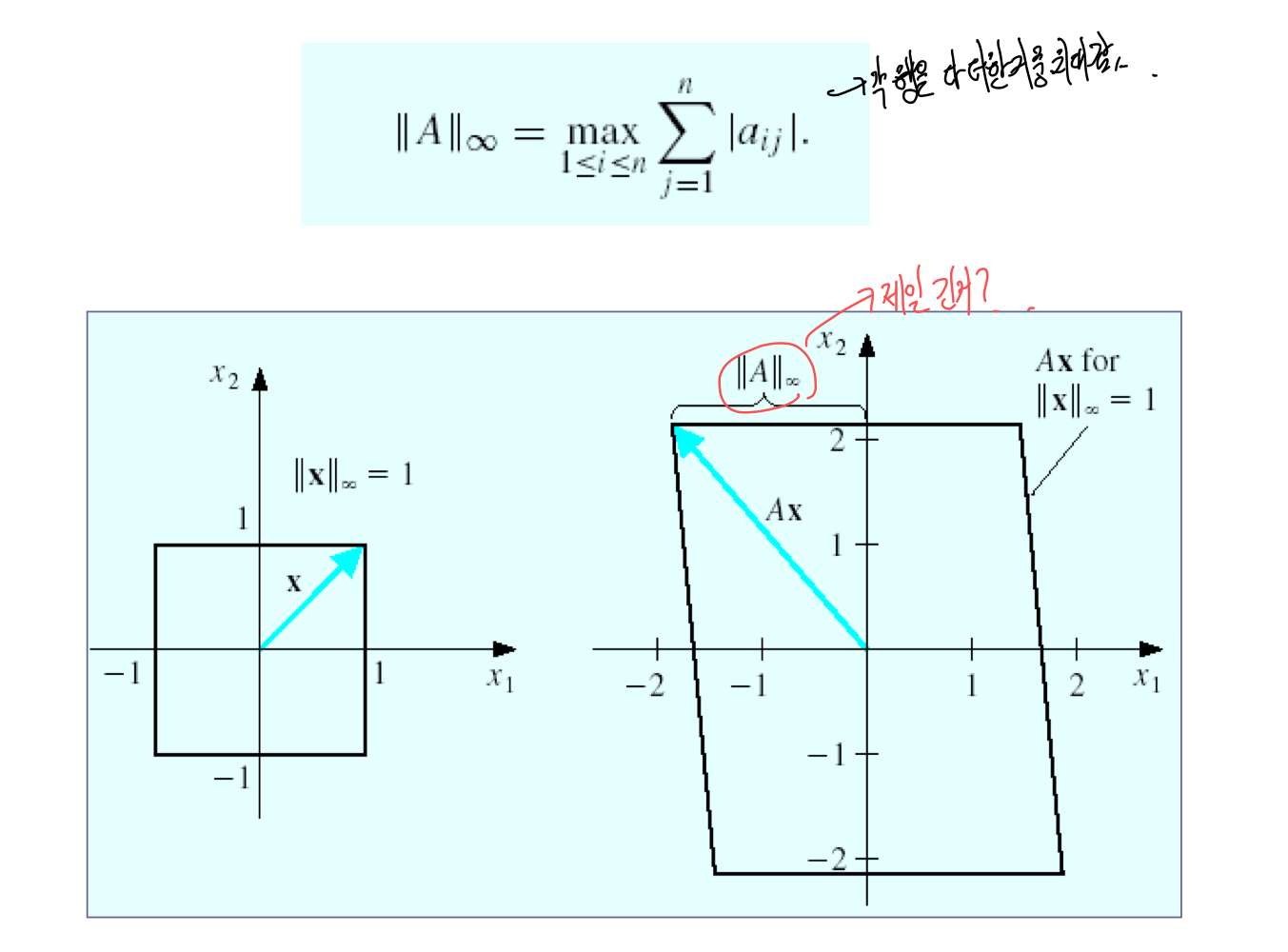
5) Natural matrix norm

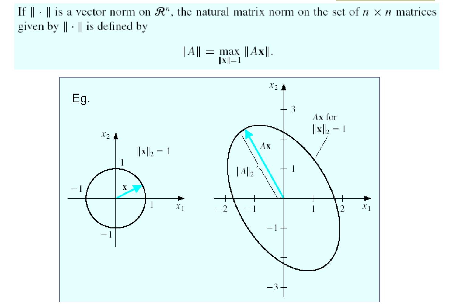
• 모든 x에 대해서 matrix A로 transform해서 얻은 가장 긴 변의 길이

6) I∞ norm of a matrix

3. Iterative linear-equations

1) Introductions

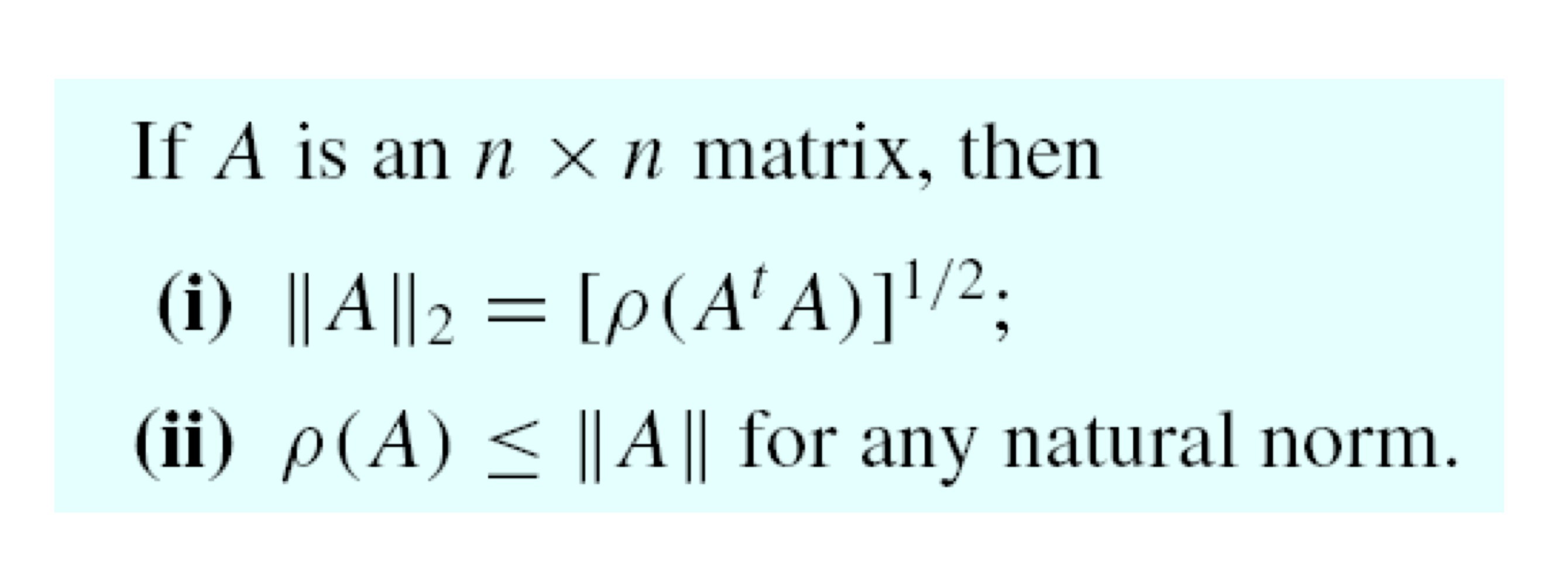
a) Spectral radius

즉 eigen value 중 최대 값

b) Convergent matrix equivalences

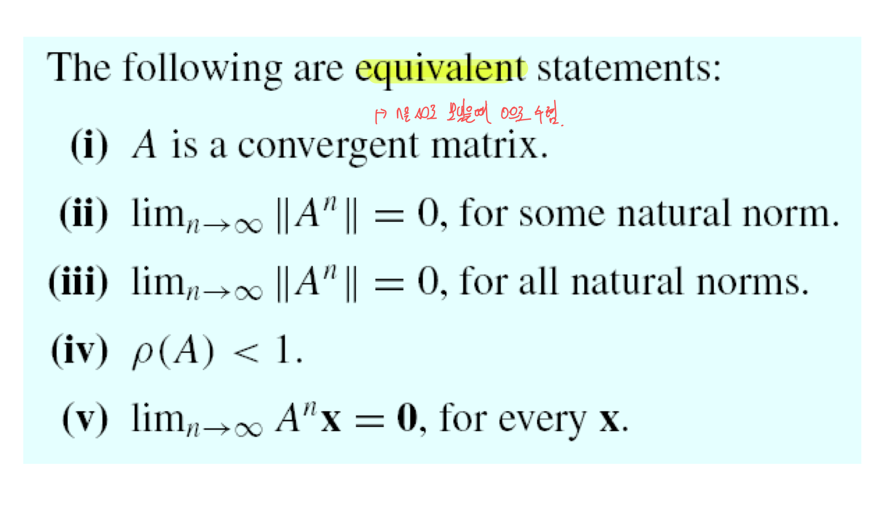
c) Convergence of a sequence

• matrix T의 eigen value와 iterative method가 수렴할 것이라고 예상하는 것 사이의 중요한 연결고리 → spectral radius
  

2) Iterative Methods - Jacobi Iteration

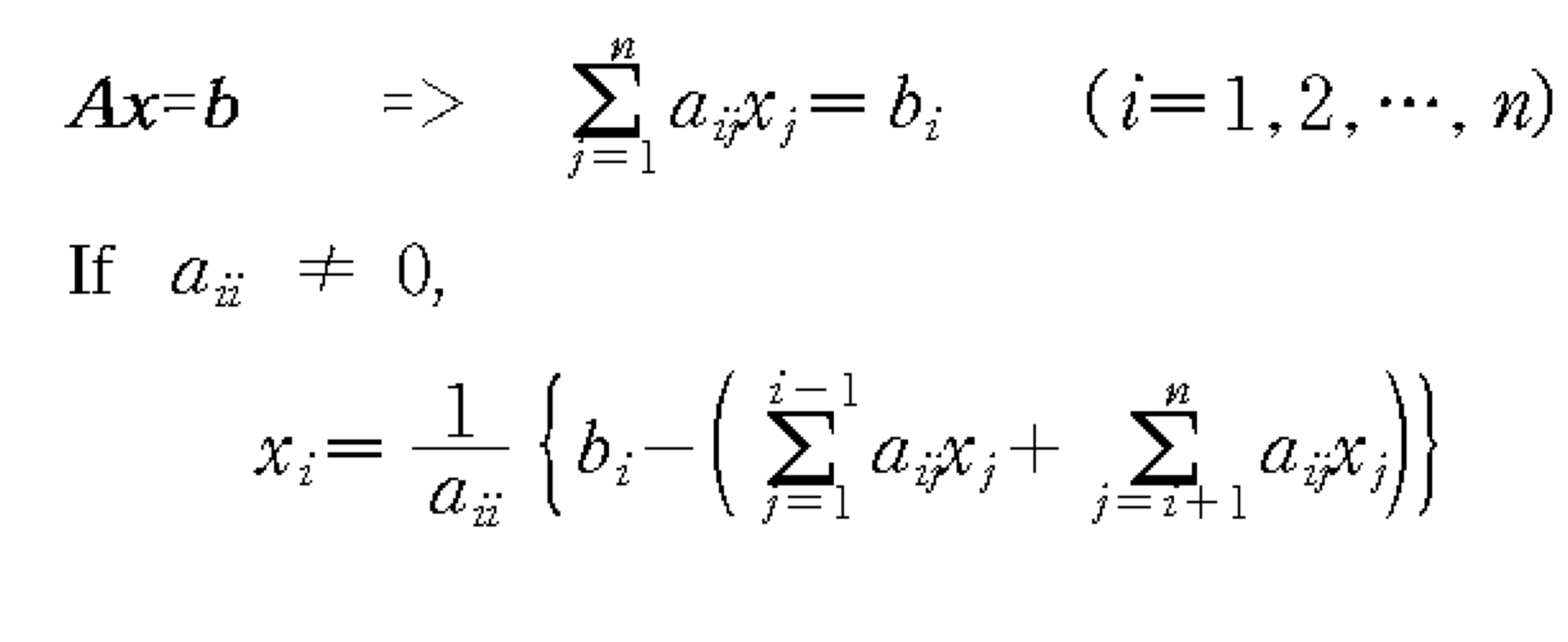
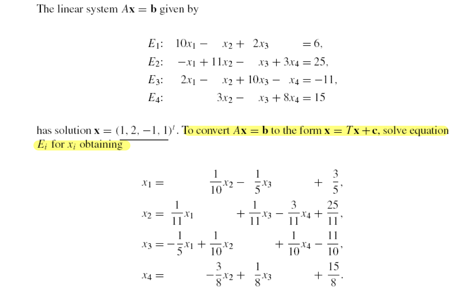
• Ax = b를 row별로 나누어 쓴다음, 전개해서 xi대한 식으로 만들면 이와 같은 관계가 나온다.

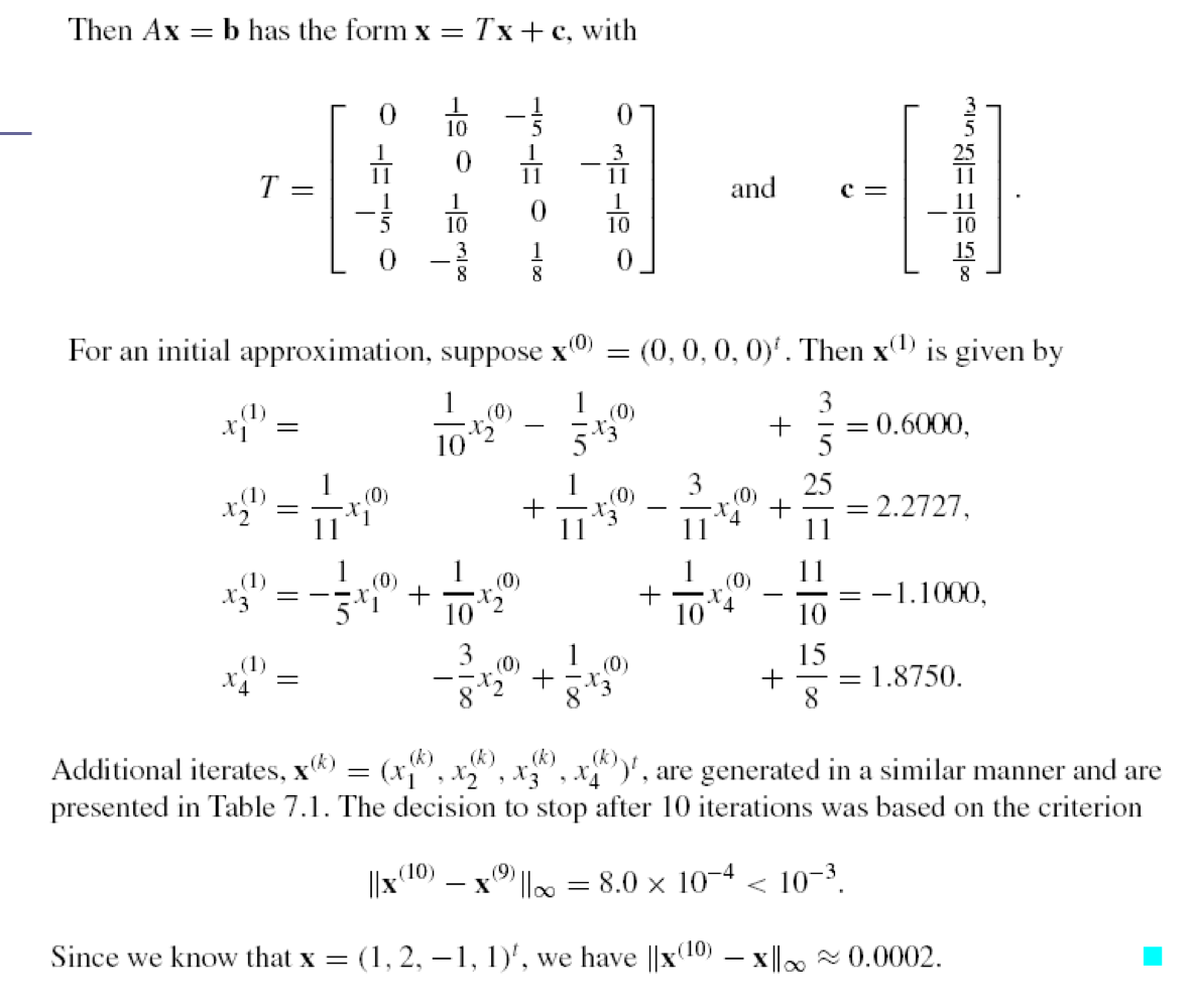
• 이를 이용해서 구한 Jacobi Iteration

a) Jacobi Iteration

• Initial guess
  • x^(0) = [x1^(0), x2^(0), … , xn^(0)]
• Convergence Condition
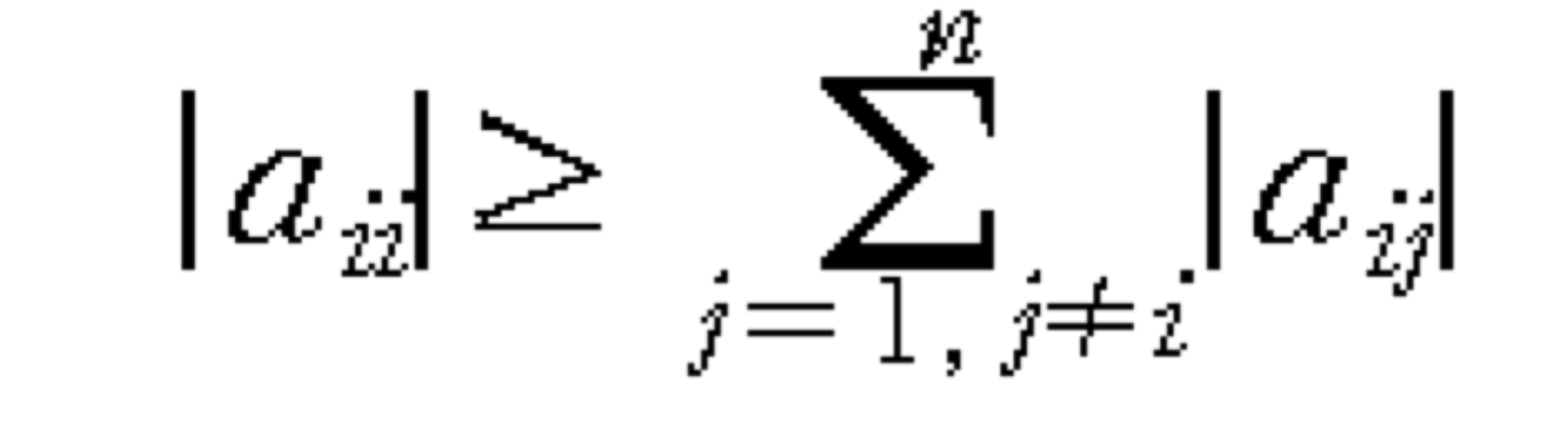
  • Jacobi iteration은 초기 추측에 관계 없이 A matrix가 diagonal dominat하다면 수렴한다.

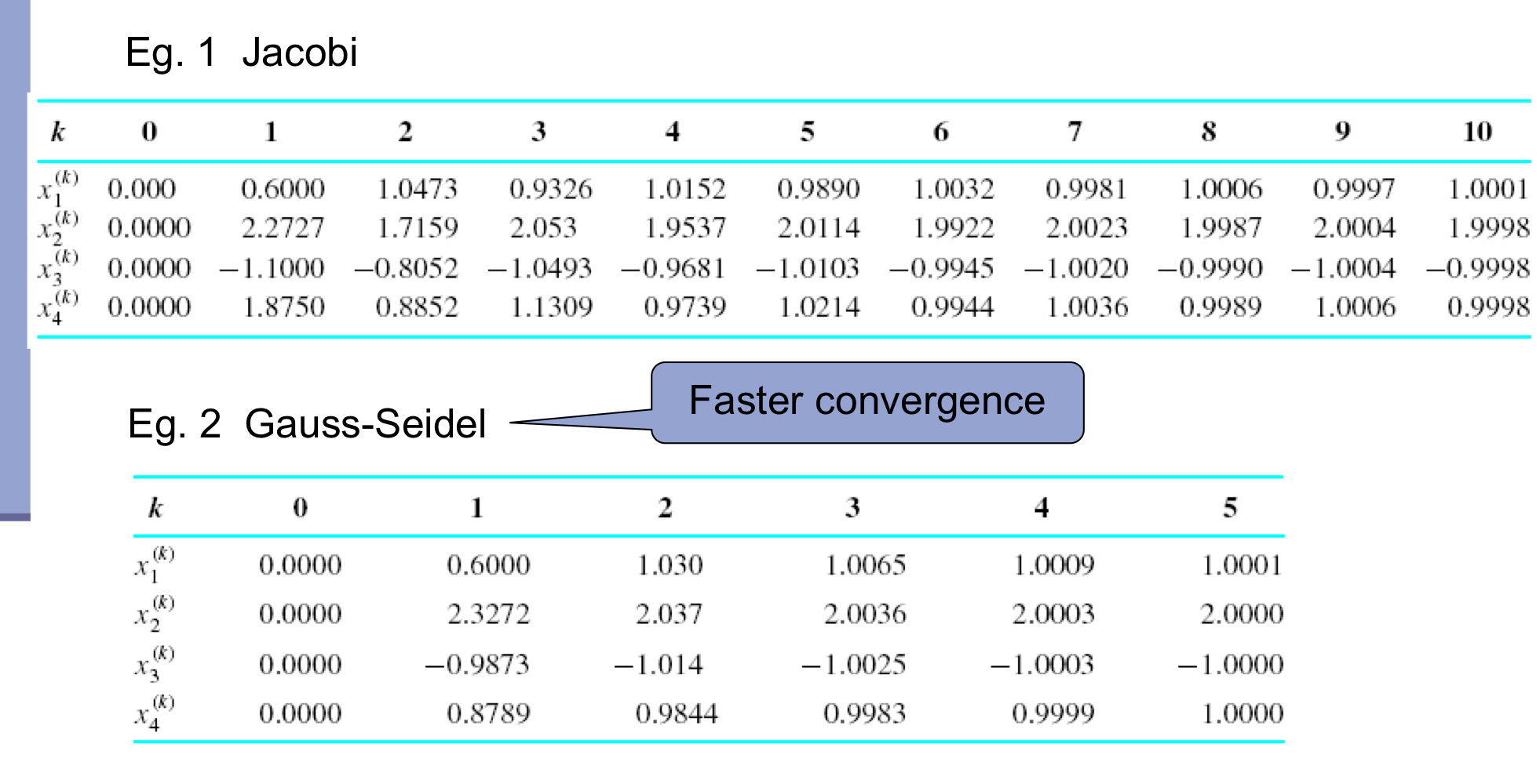
b) Eg. Jacobi Iteration

• 한계 → x1을 구할 때, x0을 사용해서 구한다. 이때, x2를 구한다고 하면, x1, x0에 대한 다음 iteration 값은 구해져 있는데 굳이 이전 값을 사용해야 할까? → Gauss-Seidel Iteration
  

2) Gauss-Seidel Iteration

• Idea
  • 최근에 업데이트 된 xi를 사용
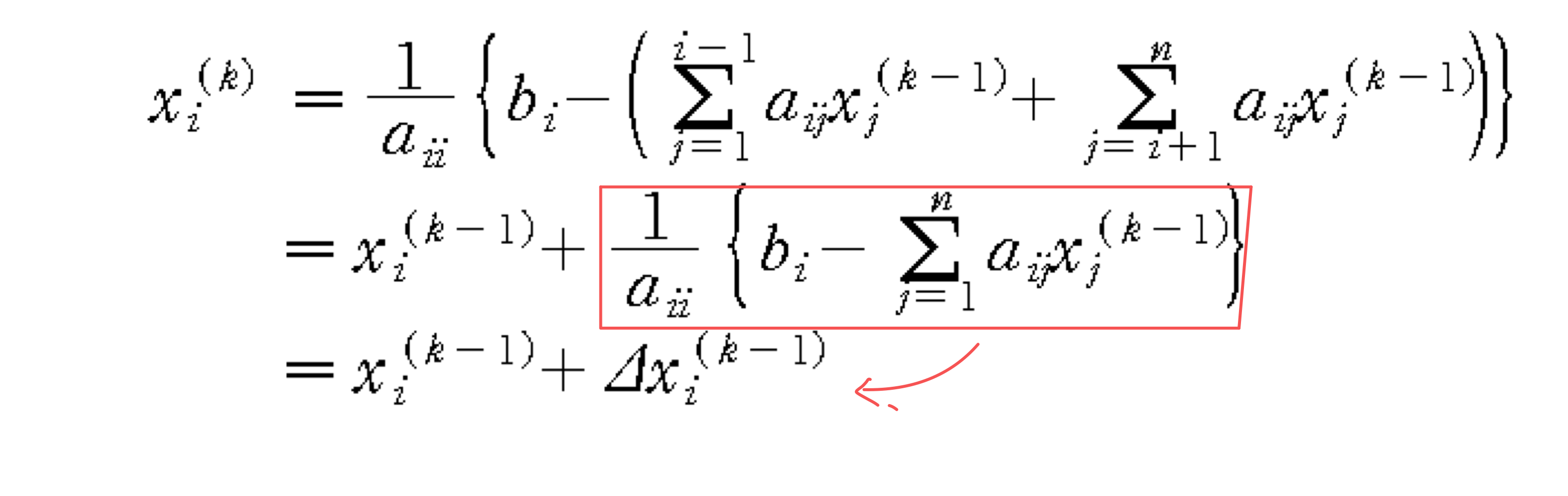
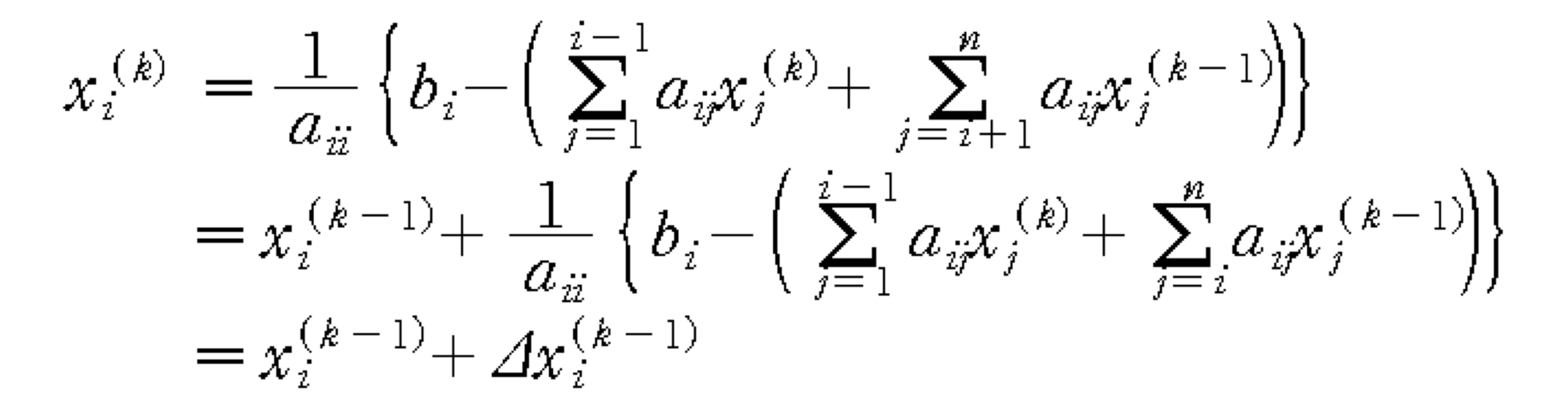
• Iteration formula (자신보다 작은 index는 업데이트 된 값 사용)

• Convergence Condition
  • Jacobi iteration과 동일 (matrix A에 대해서 diagonal dominant 해야함)
• Jacobi iteration보다 나은 이점
  • Fast Convergence

a) Eg. Gauss-Seidel iteration

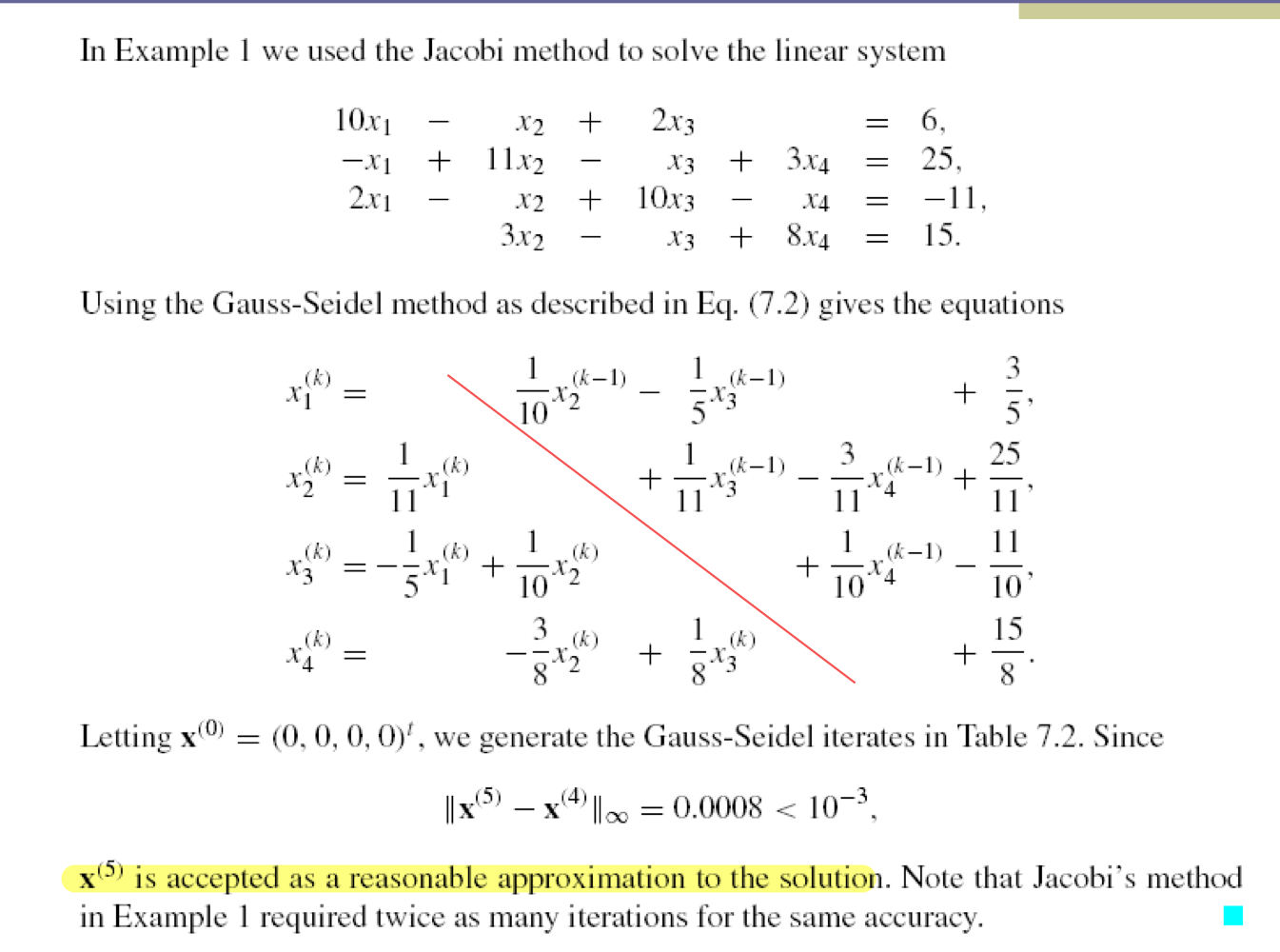
• diagonal을 중심으로 왼쪽은 k번째, 오른쪽은 k-1번째 값 사용
  • converge가 가능하다는 것을 전제로 하기에 가능하다.

b) Jacobi vs. Gauss-Seidel

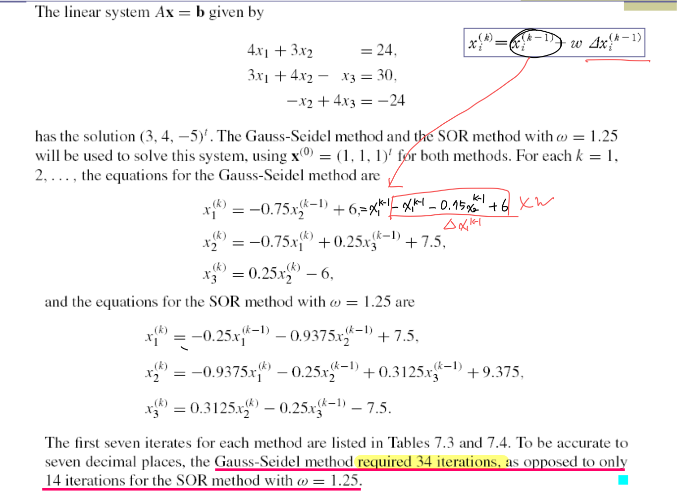
c) Variation of Gauss-Seidel Iteration

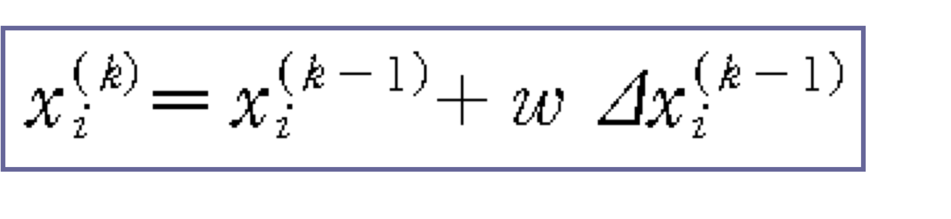
• Successive Over Relaxation (SOR)
  • 1 < w < 2
  • Fast convergence
  • linear problem에 적합하다.
  • 발산 혹은 답 근처에서 이상한 값이 발생할 수 있다.
• Successive Under Relaxation (SUR)
  • 0 < w < 1
  • Slow convergence
  • Stabel
  • Nonlinear problem에 적합하다.

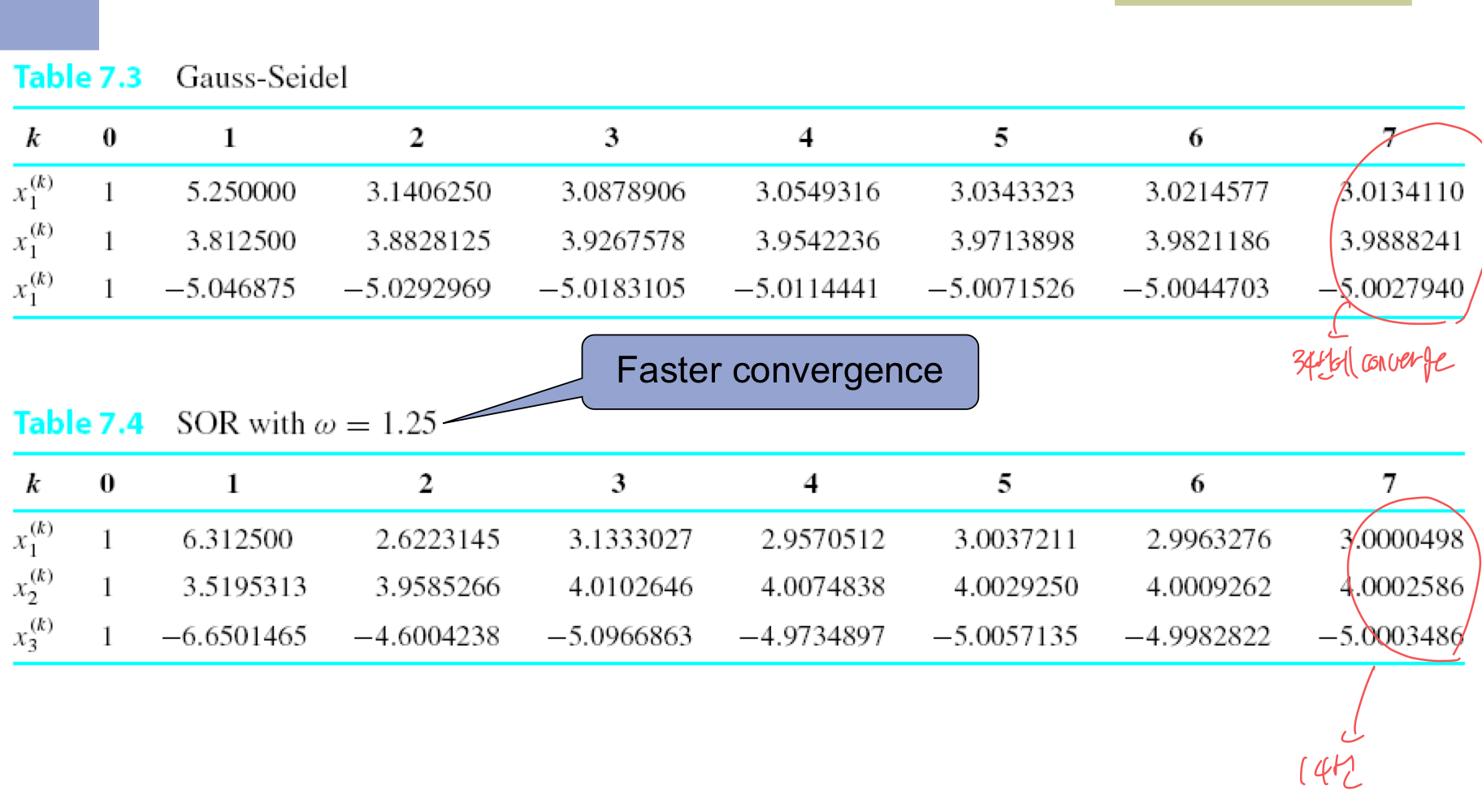
d) Eg. Gauss-Seidel vs. SOR

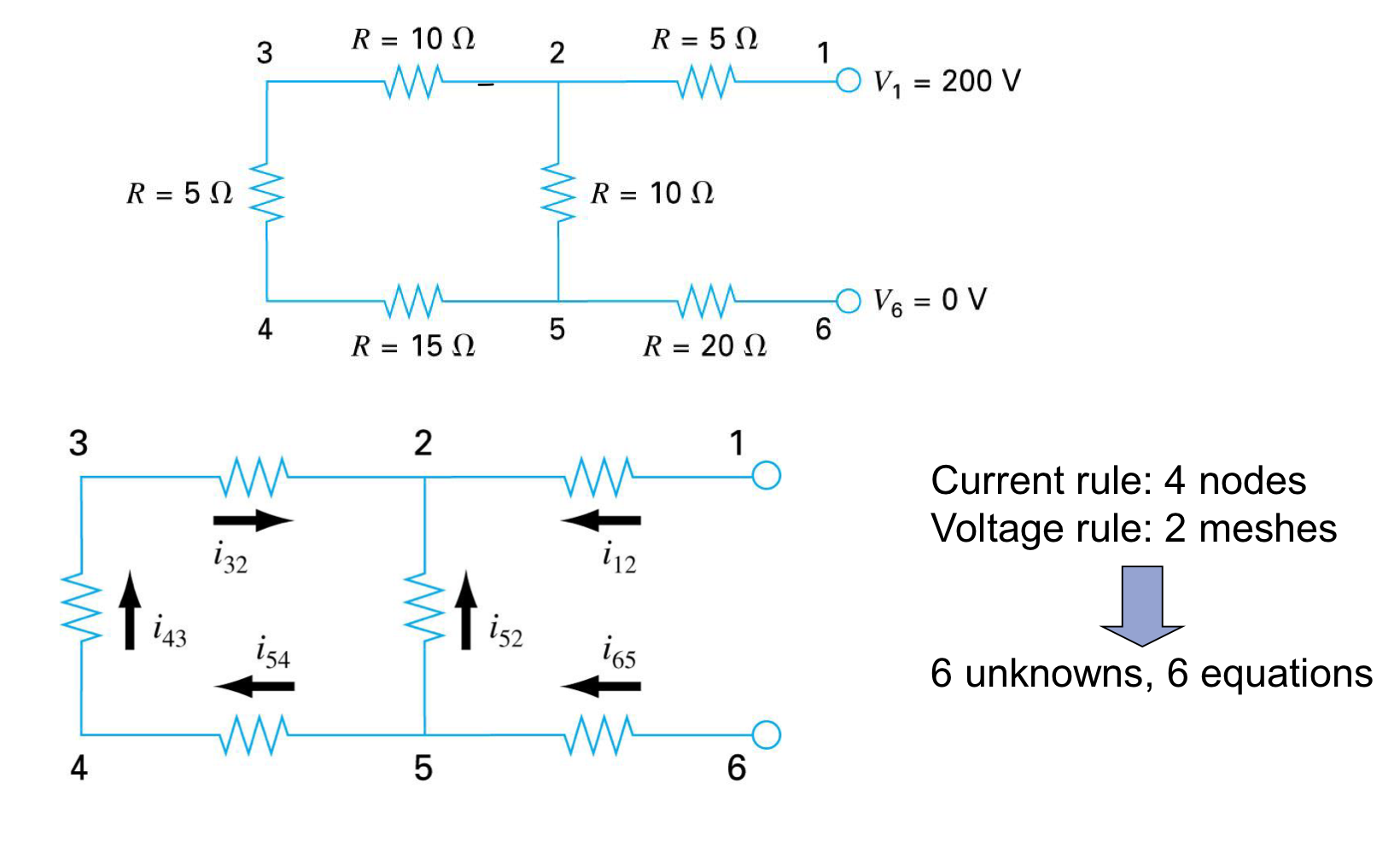
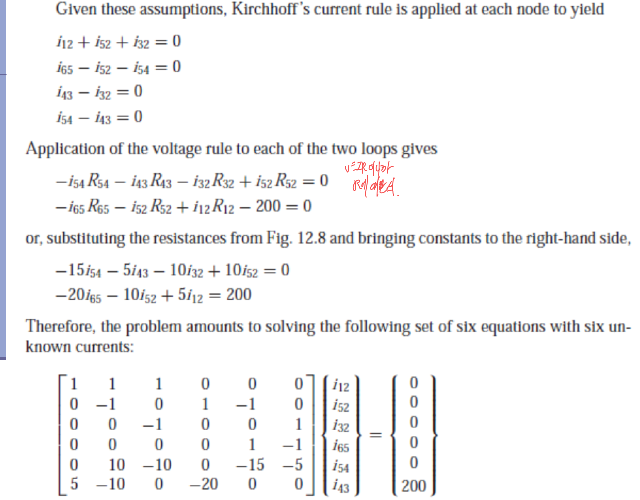
e) Application: Circuit analysis

• Krichhoff’s current and voltage law