Deep Q Network (DQN)

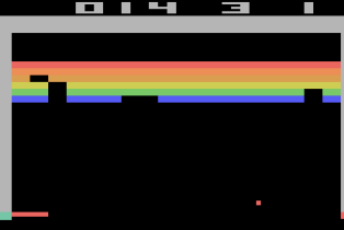
DQN은 Reinforcement Learning(RL)에 Deep Learning(DL)을 성공적으로 결합한 최초의 Deep Reinforcement Learning(DRL) 알고리즘으로 [Playing Atari with Deep Reinforcement Learning (NeurIPS 2013)]와 [Human-level control through deep reinforcement learning (Nature 2015)] 두편의 논문을 통해서 소개된 알고리즘이다.
SARSA와 Q-learning과 같은 기존의 RL 알고리즘은 각 (s,a)테이블을 기반으로 학습하였다. 하지만 이런 테이블 기반 학습은 포착가능한 상태와 선택가능한 행동의 가짓수가 많아지면 Q-table의 크기가 너무 커져서 이를 테이블로 만들어 다 저장하기엔 현실적으로 불가능 하다라는 한계점이 있었다.
DQN은 Q-table을 대신해서 $(s,a)$쌍에 대한 non-linear approximator로서 Neural Netowrk를 사용한 Q-learning기반의 알고리즘이다. 강화학습에 DL을 결합하게 되면서 아래 2가지 문제가 발생했다.

1. RL에서는 학습 데이터들 간 i.i.d.(independent and identically distributed)가정이 성립하지 않는다.

2. Target값이 계속 움직여서 학습이 수렴하지 못하고 불안정하다.

DL관점에서 i.i.d.가정이 중요한 이유는 해당 가정이 성립해야 mini-batch에 의해서 계산된 gradient가 전체 데이터 분포에 대한 gradient를 잘 대변할 수 있기 때문이다. 예를들어 시간적 상관관계가 강한 데이터 32개로 이루어진 mini-batch에서 계산된 gradient를 토대로 model의 가중치를 업데이트 한다고 가정해 보자.이때 model의 가중치는 전체 최적해를 향해 가는 것이 아닌 오직 "mini-batch가 나타내는 그 좁은 시간안에의 오차를 줄이는 방향"으로 gradient가 업데이트 된다.
이러한 문제를 [Playing Atari with Deep Reinforcement Learning (NeurIPS 2013)] 에서는 Experience Replay Buffer를 도입함으로서 해결했다. 이는 Agent가 환경과 상호작용하면서 관찰한 데이터들을 Experience Replay Buffer에 모아뒀다가 모델 업데이트 시에 random sampling하여 mini-batch를 구성함으로서 데이터 간의 시간적 상관관계를 강제로 끊어준다.

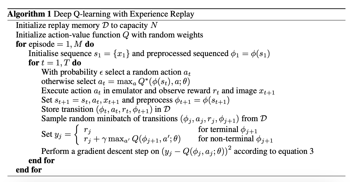
$s,a,r,s'$를 각각 현재 상태, 현재 상태에서 선택한 행동, 그에 따른 보상, 다음 상태라고 할 때 전체적인 학습 순서는 다음과 같다.

1. 환경과 상호작용하며 transition $(s,a,r,s')$를 Replay Buffer에 모은다.
2. Replay Buffer에서 random sampling하여 mini-batch를 구성한다.
3. mini-batch에 대한 gradient descent를 수행한다.

$(s,a)$에 대한 target, loss값 그리고 모델 parameter를 $\theta$라고 할 때 계산과정은 기존 DL에서의 gradient descent과정과 거의 동일하다. 이때 $\gamma$는 discount factor로 미래에 주어질 보상을 현재에 얼마나 반영할 것인지를 나타낸다. 아래는 $\theta$업데이트 과정이다.

이때 target value에 관한 미분항 $\gamma \nabla_\theta \underset{a'}{\max}Q(s',a';\theta)$는 무시하고 update를 하게 되는데 이를 Semi-Gradient method라고 한다. 그에 따른 최종 $\theta$ update식은 아래와 같다.

위 식에서 알 수 있듯이 Gradient update과정은 DL에서의 과정과 동일하다. $Q(s,a;\theta)<y$이면 $Q(s,a;\theta)$가 가장 가파르게 증가하는 방향으로 $\theta$가 update되고 반대라면 가장 가파르게 하락 하는 방향으로 $\theta$가 update된다.

Pseudo code와 수식에서 볼 수 있듯이 target 값이 predict value 값과 동일한 network$(\theta)$에 의해서 산출되는 것을 알 수 있다. 이로인해 앞선 업데이트 식에 의해서 $\theta$가 update가 되면 target value도 영향을 받게 된다. [Human-level control through deep reinforcement learning (Nature 2015)] 에서는 target network를 도입하여 앞서 언급한 문제점 중 하나인 학습 과정중 가중치가 업데이트됨에 따라서 target값도 같이 움직이는 문제점을 해결했다. 즉, 기존의 main network와 새로 도입한 target network 2개의 network를 사용했다.
Target network의 가중치 $\theta^-$는 학습 시작 시 main network의 가중치 $\theta$로 초기화 된다. 이후 $\theta^-$는 변하지 않고 고정되어 있다가 매 $C$step마다 main network의 가중치 값이 복사됨으로서 업데이트 된다. 결론적으로 기존의 algorithm에서 target value가 $\theta^-$에 대한 값으로 바뀌는 것과 $C$step마다 $\theta^- \leftarrow \theta$ 과정이 추가된 것을 제외하면 기존과 동일하다.

1. 환경과 상호작용하며 transition $(s,a,r,s')$를 Replay Buffer에 모은다.
2. Replay Buffer에서 random sampling하여 mini-batch를 구성한다.
3. mini-batch에 대한 gradient descent를 수행한다.
4. 일정한 step 마다 $\theta^- \leftarrow \theta$.