[5주차] [코드구현] Constrained Monotonic Neural Network with PyTorch

김종해·2024년 2월 10일

[2023 동계] 연구학점제

목록 보기

5/7

원문

Runje D, Shankaranarayana S, Constrained Monotonic Neural Network

참고자료

[GitHub] $~$ monotonic-nn

1. Introduction

Monotone Function을 추정하는 과정을 Isotonic Regression이라 한다. Monotone Function의 주요 특성(제약)은 Monotonicity로, 쉽게 말하면 증가함수 또는 감소함수여야 한다는 점이다. 4주차 논문은 이를 위한 기법을 고안하고 이론적 근거를 제시한다. 또한 Keras를 활용한 패키지를 제작했는데, 이를 PyTorch로 다시 제작할 것이다. 이후 Sklearn에서 제공하는 Isotonic Regression과 함께 성능을 비교할 것이다.

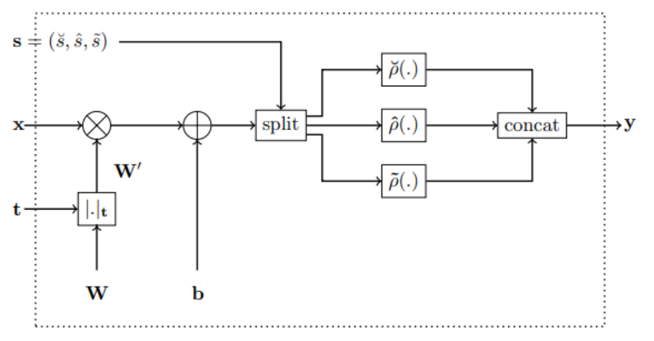
2. Monotonic Dense Block 구현

Monotone Neural Network의 핵심 부품인 다음 Monotonic Dense Block을 먼저 구현하자.

import torch
import torch.nn.functional as F
from torch.nn.parameter import Parameter
from torch.nn.modules.module import Module

# activation : relu, elu, selu, none 중 선택
class MonoBlock(Module):
    def __init__(self, in_feature:int, out_feature:int, mono_indicator = 'inc', activation = 'none', activation_partition = (0,0,1)):
        super().__init__()
        self.activation = activation
        self.activation_partition = activation_partition

        self.in_feature = in_feature
        self.out_feature = out_feature
        self.mono_indicator = mono_indicator

        self.W = Parameter(torch.randn(self.in_feature, self.out_feature))
        self.b = Parameter(torch.randn(self.out_feature))

    def get_activation(self):
        convex = getattr(F, self.activation)
        def concave(x):
            return -convex(-x)
        def saturated(x):
            plus = -convex(-x+torch.ones_like(x)) + convex(torch.ones_like(x))
            minus = convex(x+torch.ones_like(x)) - convex(torch.ones_like(x))
            return torch.where(x >= 0, plus, minus)
        return convex, concave, saturated

    def activation_index(self, x):
        if sum(self.activation_partition) != 1:
            raise ValueError(f"sum of activation_partition must be 1")
        if len(self.activation_partition) != 3:
            raise ValueError(f"length of activation_partition must be 3")

        convex_num = int(self.activation_partition[0] * len(x.T))
        concave_num = int(self.activation_partition[1] * len(x.T))
        return convex_num, convex_num+concave_num, len(x.T)

    def forward(self, x):
        if len(x.shape) == 1:
            x = x.reshape(-1, 1)
        if self.mono_indicator == 'inc':
            self.mono_indicator = torch.ones(x.shape[1])
        if x.shape[1] != self.in_feature:
            raise ValueError(f"matrix multiplication cannot be implemented : {x.shape[0]}x{x.shape[1]} and {self.in_feature}x{self.out_feature}")
        if len(self.mono_indicator) != self.in_feature:
            raise ValueError(f"number of variable does not match : {len(self.mono_indicator)} and {self.in_feature}")

        mono_oper = torch.tensor(self.mono_indicator).reshape(-1, 1) * torch.abs(self.W)
        W_oper = torch.where(torch.abs(mono_oper) >= torch.abs(self.W), mono_oper, self.W)
        x = torch.matmul(x, W_oper) + self.b

        convex_idx, concave_idx, saturated_idx = self.activation_index(x)
        if self.activation == 'none':
            out = torch.cat([x.T[:convex_idx], x.T[convex_idx:concave_idx], x.T[concave_idx:saturated_idx]], dim=0)
        else:
            convex_act, concave_act, saturated_act = self.get_activation()
            out = torch.cat([convex_act(x.T[:convex_idx]), concave_act(x.T[convex_idx:concave_idx]), saturated_act(x.T[concave_idx:saturated_idx])], dim=0).T

        return out

구현해야할 핵심 기능은 총 3가지다.

get_activation(self)
- zero-centered, monotonically increasing, convex, lower-bounded인 Activation Function $\breve{\rho}$ 을 입력했을 때, $\hat{\rho}$ , $\tilde{\rho}$ 를 반환하는 메소드다.
- activation은 $\breve{\rho}$ 를 지정하는 것으로, 'none'이면 항등함수를, 그 외는 torch.nn.functional에서 해당 이름의 함수를 가져온다.
activation_index(self, x)
- 아핀 변환된 Input vector( $=|\mathbf{W^T}|_t\cdot\mathbf{x+b}$ )가 3분할될 index를 반환하는 메소드다.
- activation_partition은 $\breve{s}, \hat{s}, \tilde{s}$ 의 비율을 나타낸다.
forward(self, x)
- $\mathbf{x} \rightarrow \rho^S(|\mathbf{W^T}|_t\cdot\mathbf{x+b})$ 를 수행하는 메소드다.
- mono_indicator는 Input vector의 각 변수의 증가/감소/제약없음 여부를 결정하는 array이다. mono_indicator에 따라 $\mathbf{W} \rightarrow |\mathbf{W^T}|_t$ 를 계산한다.
- activation_index에 따라 $\breve{\rho}, \hat{\rho}, \tilde{\rho}$ 에 적용시키고, 다시 하나의 벡터로 합친다.

Activation Function $\breve{\rho}$ 에 따라 $\hat{\rho}, \tilde{\rho}$ 가 잘 반환되는지 확인해보자.

# convex, concave, non-convex-concave 시각화
import matplotlib.pyplot as plt
fig = plt.figure()

x = torch.linspace(-2, 2, steps=201)

# ReLU 시각화
convex_relu, concave_relu, saturated_relu = MonoBlock(1, 3, [1], activation='relu').get_activation()

ax1 = fig.add_subplot(231)
ax4 = fig.add_subplot(234)

ax1.plot(x, convex_relu(x))
ax4.plot(x, convex_relu(x))
ax4.plot(x, concave_relu(x))
ax4.plot(x, saturated_relu(x).detach())

# ELU 시각화
convex_elu, concave_elu, saturated_elu = MonoBlock(1, 3, [1], activation='elu').get_activation()

ax2 = fig.add_subplot(232)
ax5 = fig.add_subplot(235)

ax2.plot(x, convex_elu(x))
ax5.plot(x, convex_elu(x))
ax5.plot(x, concave_elu(x))
ax5.plot(x, saturated_elu(x).detach())

# SeLU 시각화
convex_selu, concave_selu, saturated_selu = MonoBlock(1, 3, [1], activation='selu').get_activation()

ax3 = fig.add_subplot(233)
ax6 = fig.add_subplot(236)

ax3.plot(x, convex_selu(x))
ax6.plot(x, convex_selu(x))
ax6.plot(x, concave_selu(x))
ax6.plot(x, saturated_selu(x).detach())

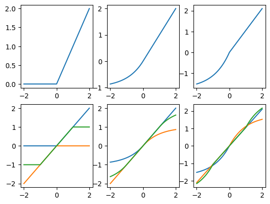
논문에서 제시한 다음 그림과 동일한 결과를 얻을 수 있었다.

3. Monotone Neural Network 구현

Monotonic Dense Block을 쌓아 Monotone Neural Network를 구현하자.

import torch.nn as nn
import torch.nn.functional as F

class MonoNet(nn.Module):
    def __init__(self):
        super().__init__()
        self.mono = nn.Sequential(
            MonoBlock(1, 32, mono_indicator=[1], activation='elu', activation_partition=(0, 0, 1)),
            MonoBlock(32, 16, activation='elu', activation_partition=(0, 0, 1)),
            MonoBlock(16, 8, activation='elu', activation_partition=(0, 0, 1)),
            MonoBlock(8, 4, activation='elu', activation_partition=(0, 0, 1)),
            MonoBlock(4, 1)
        )

    def forward(self, x):
        return self.mono(x)

mono_indicator의 길이는 Input vector의 차원과 같아야 한다. $i$ 번째 indicator가 $i$ 번째 변수의 증감 여부를 결정하기 때문이다.
layer 수, 각 layer의 입력/출력 벡터 차원은 자유롭게 설정할 수 있다.

4. Monotone Neural Network 성능비교

모의함수로부터 데이터를 생성하고, 이를 PyTorch 모델, Keras 모델, Sklearn 모델에 학습시켜 예측결과를 비교하자. 성능은 test data의 MSE로 나타낼 것이다.

import numpy as np

# Reproduce를 위한 seed 고정
random_seed = 42
torch.manual_seed(random_seed)
np.random.seed(random_seed)

# 데이터 생성 _ train, valid, test
def data_generate(num_sample, noise):
    X = np.random.uniform(-1, 5, num_sample)
    Y = np.exp(X - 2 + np.sin(X)) + noise * np.random.normal(0, 0.1, num_sample)
    return torch.tensor(X, dtype=torch.float), torch.tensor(Y, dtype=torch.float)

train_x, train_y = data_generate(800, 0.8)
valid_x, valid_y = data_generate(100, 0)
test_x, test_y = data_generate(100, 0)

모의함수는 $y=e^{x-2+\sin x}$ 이고, 증가함수다. train data에는 노이즈를 첨가하고, valid, test data는 노이즈를 첨가하지 않았다.

PyTorch 모델 학습

# PyTorch 모델 학습
my_param = {'learning_rate' : 0.01,
            'num_epoch' : 2000}

criterion = nn.MSELoss()
optimizer = torch.optim.Adam(model.parameters(), lr=my_param['learning_rate'])
best_valid_loss_torch = 10**9

for epoch in range(1, my_param['num_epoch']+1):
    model.train()

    output = model(train_x)
    train_loss = criterion(output, train_y)

    optimizer.zero_grad()
    train_loss.backward()
    optimizer.step()

    with torch.no_grad():
        model.eval()
        if epoch % 50 == 0:
            valid_output = model(valid_x)
            valid_loss = criterion(valid_output, valid_y)
            print(f"    [Epoch {epoch}] Valid loss : {valid_loss}")

            if best_valid_loss_torch > valid_loss:
                best_valid_loss_torch = valid_loss

print(f"[PyTorch] Best valid loss : {best_valid_loss_torch}")

Keras 모델 학습

# Keras 모델 설계
from tensorflow.keras import Sequential
from tensorflow.keras.layers import Dense, Input
from airt.keras.layers import MonoDense
from tensorflow.keras.optimizers import Adam

model_keras = Sequential()

model_keras.add(Input(shape=(1,)))
model_keras.add(
    MonoDense(512, activation="elu", monotonicity_indicator=[1]))
model_keras.add(
    MonoDense(512, activation="elu"))
model_keras.add(
    MonoDense(512, activation="elu"))
model_keras.add(
    MonoDense(512, activation="elu"))
model_keras.add(
    MonoDense(1))

optimizer_keras = Adam(learning_rate=my_param['learning_rate'])
model_keras.compile(optimizer=optimizer_keras, loss="mse")

model_keras.fit(
    x=np.array(train_x), y=np.array(train_y), batch_size=10000, validation_data=(np.array(valid_x), np.array(valid_y)), epochs=2000
)

Sklearn 모델 학습

# SKlearn 모델 설계

from sklearn.isotonic import IsotonicRegression
iso_reg = IsotonicRegression().fit(train_x, train_y)

모델 평가

# PyTorch 모델 평가
test_pred = model(test_x)

fig = plt.figure()
fig.set_figwidth(25)
ax1 = fig.add_subplot(131)

ax1.scatter(test_x.detach(), test_y.detach(), color='r')
ax1.scatter(test_x.detach(), test_pred.detach(), color='b')
ax1.set_title('PyTorch')
ax1.text(-1, 6.5, f"MSE : {criterion(test_y, test_pred)}")
ax1.text(-1, 6, f"Param : {sum(p.numel() for p in model.parameters() if p.requires_grad)}")


# Keras 모델 평가
test_pred_keras = model_keras.predict(x=np.array(test_x))
ax2 = fig.add_subplot(132)

ax2.scatter(test_x.detach(), test_y.detach(), color='r')
ax2.scatter(test_x.detach(), test_pred_keras, color='b')
ax2.set_title('Keras')
ax2.text(-1, 6.5, f"MSE : {criterion(test_y, torch.tensor(test_pred_keras))}")
ax2.text(-1, 6, f"Param : {model_keras.count_params()}")

# Sklearn 모델평가
test_pred_iso = iso_reg.predict(test_x)
ax3 = fig.add_subplot(133)

ax3.scatter(test_x.detach(), test_y.detach(), color='r')
ax3.scatter(test_x.detach(), test_pred_iso, color='b')
ax3.set_title('Sklearn')
ax3.text(-1, 6.5, f"MSE : {criterion(test_y, torch.tensor(test_pred_iso))}")
ax3.text(-1, 6, f"Param : -")

test data에 대한 예측 결과는 다음과 같다. 붉은 점은 True 함수에 의한 함숫값, 푸른 점은 모델의 예측값이다.

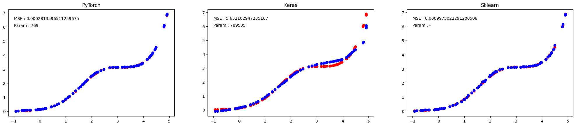
PyTorch 모델은 Sklearn 모델과 거의 유사한, 최고성능을 냈음을 확인할 수 있다.
Keras 모델에 비해 PyTorch 모델은 적은 파라미터로도 더 좋은 성능을 냈음을 확인할 수 있다.

PyTorch 모델이 단조성을 만족하는지 확인해보자.

# 단조성 검증 _ PyTorch
sort_idx_x = np.argsort(test_x.detach().numpy())
sort_idx_pred = np.argsort(test_pred.detach().numpy()[0])
np.all(sort_idx_x == sort_idx_pred)