관련논문
- Runje D, Shankaranarayana S, Constrained Monotonic Neural Network
- Choi Y, Semi-Parametric Contextual Pricing Algorithm using Cox Proportional
Hazards Model
1. Introduction
Monotone Neural Network를 살펴보고 구현한 이유는, 이를 이용하여 누적분포함수(CDF)를 추정하기 위함이다. 모든 CDF는 monotone increasing이고 bounded(0~1)이므로, Monotone Neural Network의 결과값이 0 이상 1이하의 값을 갖도록 기법을 추가할 것이다.
또한 원점을 지나는 Monotone Neural Network를 구현할 것이다. 이는 Cox Regression에서 Cumulative Hazard rate를 추정하기 위함이다. 자세한 내용은 7주차에서 소개할 것이다.
현재 단계에서는 Input/Output이 모두 1차원인 증가함수만 다룬다. 각 기법은 고차원의 경우로 잘 확장될 수 있을 것이다.
2. Bounded Monotone Neural Network
모델의 결과값이 0 이상(혹은 초과) 1 이하(혹은 미만)로 만들기 위해, 인 증가함수를 합성할 것이다. 대표적으로는 Sigmoid 함수, Tanh 함수(적절히 scaling한다면) 등이 있다.
우선 Monotonic Dense Block을 가져오자.
import torch
import torch.nn as nn
import torch.nn.functional as F
from torch.nn.parameter import Parameter
from torch.nn.modules.module import Module

import numpy as np
import matplotlib.pyplot as plt

# MonoBlock 구현
## activation : relu, elu, selu, none 중 선택
class MonoBlock(Module):
    def __init__(self, in_feature:int, out_feature:int, mono_indicator = 'inc', activation = 'none', activation_partition = (0,0,1)):
        super().__init__()
        self.activation = activation
        self.activation_partition = activation_partition

        self.in_feature = in_feature
        self.out_feature = out_feature
        self.mono_indicator = mono_indicator

        self.W = Parameter(torch.randn(self.in_feature, self.out_feature))
        self.b = Parameter(torch.randn(self.out_feature))

    def get_activation(self):
        convex = getattr(F, self.activation)
        def concave(x):
            return -convex(-x)
        def saturated(x):
            plus = -convex(-x+torch.ones_like(x)) + convex(torch.ones_like(x))
            minus = convex(x+torch.ones_like(x)) - convex(torch.ones_like(x))
            return torch.where(x >= 0, plus, minus)
        return convex, concave, saturated

    def activation_index(self, x):
        if sum(self.activation_partition) != 1:
            raise ValueError(f"sum of activation_partition must be 1")
        if len(self.activation_partition) != 3:
            raise ValueError(f"length of activation_partition must be 3")

        convex_num = int(self.activation_partition[0] * len(x.T))
        concave_num = int(self.activation_partition[1] * len(x.T))
        return convex_num, convex_num+concave_num, len(x.T)

    def forward(self, x):
        if len(x.shape) == 1:
            x = x.reshape(-1, 1)
        if self.mono_indicator == 'inc':
            self.mono_indicator = torch.ones(x.shape[1])
        if x.shape[1] != self.in_feature:
            raise ValueError(f"matrix multiplication cannot be implemented : {x.shape[0]}x{x.shape[1]} and {self.in_feature}x{self.out_feature}")
        if len(self.mono_indicator) != self.in_feature:
            raise ValueError(f"number of variable does not match : {len(self.mono_indicator)} and {self.in_feature}")

        mono_oper = torch.tensor(self.mono_indicator).reshape(-1, 1) * torch.abs(self.W)
        W_oper = torch.where(torch.abs(mono_oper) >= torch.abs(self.W), mono_oper, self.W)
        x = torch.matmul(x, W_oper) + self.b

        convex_idx, concave_idx, saturated_idx = self.activation_index(x)
        if self.activation == 'none':
            out = torch.cat([x.T[:convex_idx], x.T[convex_idx:concave_idx], x.T[concave_idx:saturated_idx]], dim=0)
        else:
            convex_act, concave_act, saturated_act = self.get_activation()
            out = torch.cat([convex_act(x.T[:convex_idx]), concave_act(x.T[convex_idx:concave_idx]), saturated_act(x.T[concave_idx:saturated_idx])], dim=0).T

        return out
Monotone Neural Network를 만들고, 가장 마지막에 Sigmoid 함수롸 Tanh 함수를 합성할 것이다. Tanh 함수는 함숫값이 0과 1 사이에 오도록 하기 위해 로 사용한다.
# Bdd(0~1) MonoNet 구현
## Sigmoid
class BddMonoNet_Sig(nn.Module):
    def __init__(self):
        super().__init__()
        self.mono = nn.Sequential(
            MonoBlock(1, 32, mono_indicator=[1], activation='elu', activation_partition=(0, 0, 1)),
            MonoBlock(32, 16, activation='elu', activation_partition=(0, 0, 1)),
            MonoBlock(16, 8, activation='elu', activation_partition=(0, 0, 1)),
            MonoBlock(8, 4, activation='elu', activation_partition=(0, 0, 1)),
            MonoBlock(4, 1)
        )

    def forward(self, x):
        return torch.sigmoid(self.mono(x))

## Tanh
class BddMonoNet_Tanh(nn.Module):
    def __init__(self):
        super().__init__()
        self.mono = nn.Sequential(
            MonoBlock(1, 32, mono_indicator=[1], activation='elu', activation_partition=(0, 0, 1)),
            MonoBlock(32, 16, activation='elu', activation_partition=(0, 0, 1)),
            MonoBlock(16, 8, activation='elu', activation_partition=(0, 0, 1)),
            MonoBlock(8, 4, activation='elu', activation_partition=(0, 0, 1)),
            MonoBlock(4, 1)
        )

    def forward(self, x):
        return 0.5 * torch.tanh(self.mono(x)) + 0.5
모델 검증
위 기법이 잘 작동하는지 실험을 통해 검증해보자. 두 개의 모의함수로부터 데이터를 생성하고, 각 모델에 학습시켜 예측 결과를 관찰할 것이다.
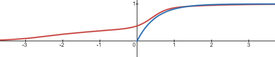
- 붉은 그래프 :
- 푸른 그래프 :
  # Reproduce를 위한 seed 고정
random_seed = 42
torch.manual_seed(random_seed)
np.random.seed(random_seed)

# 데이터 생성 _ train, valid, test
def data_generate1(num_sample, noise):
    X = np.random.uniform(-4, 4, num_sample)
    Y1 = 0.3 / (1 + np.exp(-X))
    Y2 = 0.5 / (1 + np.exp(-5*X+2))
    Y3 = 0.2 / (1 + np.exp(-2*X-5))
    Y = Y1 + Y2 + Y3 + noise * np.random.normal(0, 1, num_sample)
    return torch.tensor(X, dtype=torch.float), torch.tensor(Y, dtype=torch.float)

def data_generate2(num_sample, noise):
    X = np.random.uniform(0, 8, num_sample)
    Y = 1 - np.exp(-2*X) + noise * np.random.normal(0, 1, num_sample)
    return torch.tensor(X, dtype=torch.float), torch.tensor(Y, dtype=torch.float)

train_x1, train_y1 = data_generate1(800, 0.1)
train_x2, train_y2 = data_generate2(800, 0.1)

valid_x1, valid_y1 = data_generate1(100, 0)
valid_x2, valid_y2 = data_generate2(100, 0)

test_x1, test_y1 = data_generate1(100, 0)
test_x2, test_y2 = data_generate2(100, 0)
생성한 데이터로 두 모델을 학습시킨다.
# 모델학습
## BddMonoNet_Sig
my_param_sig = {'learning_rate' : 0.001,
            'num_epoch' : 10000}

## 1번 데이터
model_sig1 = BddMonoNet_Sig()
criterion = nn.MSELoss()
optimizer = torch.optim.Adam(model_sig1.parameters(), lr=my_param_sig['learning_rate'])
best_valid_loss_torch = 10**9

for epoch in range(1, my_param_sig['num_epoch']+1):
    model_sig1.train()

    output = model_sig1(train_x1)
    train_loss = criterion(output, train_y1)

    optimizer.zero_grad()
    train_loss.backward()
    optimizer.step()

    with torch.no_grad():
        model_sig1.eval()
        if epoch % 500 == 0:
            valid_output = model_sig1(valid_x1)
            valid_loss = criterion(valid_output, valid_y1)
            print(f"    [Epoch {epoch}] Valid loss : {valid_loss}")

            if best_valid_loss_torch > valid_loss:
                best_valid_loss_torch = valid_loss

print(f"[PyTorch] Best valid loss : {best_valid_loss_torch}")


# 2번 데이터
model_sig2 = BddMonoNet_Sig()
criterion = nn.MSELoss()
optimizer = torch.optim.Adam(model_sig2.parameters(), lr=my_param_sig['learning_rate'])
best_valid_loss_torch = 10**9

for epoch in range(1, my_param_sig['num_epoch']+1):
    model_sig2.train()

    output = model_sig2(train_x2)
    train_loss = criterion(output, train_y2)

    optimizer.zero_grad()
    train_loss.backward()
    optimizer.step()

    with torch.no_grad():
        model_sig2.eval()
        if epoch % 500 == 0:
            valid_output = model_sig2(valid_x2)
            valid_loss = criterion(valid_output, valid_y2)
            print(f"    [Epoch {epoch}] Valid loss : {valid_loss}")

            if best_valid_loss_torch > valid_loss:
                best_valid_loss_torch = valid_loss

print(f"[PyTorch] Best valid loss : {best_valid_loss_torch}")
# 모델학습
## BddMonoNet_Tanh
my_param_tanh = {'learning_rate' : 0.001,
'num_epoch' : 10000}
# 1번 데이터
model_tanh1 = BddMonoNet_Tanh()
criterion = nn.MSELoss()
optimizer = torch.optim.Adam(model_tanh1.parameters(), lr=my_param_tanh['learning_rate'])
best_valid_loss_torch = 10**9
for epoch in range(1, my_param_tanh['num_epoch']+1):
model_tanh1.train()
output = model_tanh1(train_x1)
train_loss = criterion(output, train_y1)
optimizer.zero_grad()
train_loss.backward()
optimizer.step()
with torch.no_grad():
model_tanh1.eval()
if epoch % 500 == 0:
valid_output = model_tanh1(valid_x1)
valid_loss = criterion(valid_output, valid_y1)
print(f" [Epoch {epoch}] Valid loss : {valid_loss}")
if best_valid_loss_torch > valid_loss:
best_valid_loss_torch = valid_loss
print(f"[PyTorch] Best valid loss : {best_valid_loss_torch}")
# 2번 데이터
model_tanh2 = BddMonoNet_Tanh()
criterion = nn.MSELoss()
optimizer = torch.optim.Adam(model_tanh2.parameters(), lr=my_param_tanh['learning_rate'])
best_valid_loss_torch = 10**9
for epoch in range(1, my_param_tanh['num_epoch']+1):
model_tanh2.train()
output = model_tanh2(train_x2)
train_loss = criterion(output, train_y2)
optimizer.zero_grad()
train_loss.backward()
optimizer.step()
with torch.no_grad():
model_tanh2.eval()
if epoch % 500 == 0:
valid_output = model_tanh2(valid_x2)
valid_loss = criterion(valid_output, valid_y2)
print(f" [Epoch {epoch}] Valid loss : {valid_loss}")
if best_valid_loss_torch > valid_loss:
best_valid_loss_torch = valid_loss
print(f"[PyTorch] Best valid loss : {best_valid_loss_torch}")test data에 대한 각 모델의 예측 결과는 다음과 같다. 붉은 점은 True 함수의 함숫값, 푸른 점은 모델의 예측 결과값이다.
# BddMonoNet_Sig, BddMonoNet_Tanh 모델 평가
test_pred_sig1 = model_sig1(test_x1)
test_pred_sig2 = model_sig2(test_x2)
test_pred_tanh1 = model_tanh1(test_x1)
test_pred_tanh2 = model_tanh2(test_x2)

# 결과 시각화
fig_cdf_test = plt.figure()
fig_cdf_test.set_figwidth(15)

ax_cdf_test_sig1 = fig_cdf_test.add_subplot(221)
ax_cdf_test_sig1.scatter(test_x1.detach(), test_y1.detach(), color='r')
ax_cdf_test_sig1.scatter(test_x1.detach(), test_pred_sig1[0].detach(), color='b')

ax_cdf_test_sig2 = fig_cdf_test.add_subplot(222)
ax_cdf_test_sig2.scatter(test_x2.detach(), test_y2.detach(), color='r')
ax_cdf_test_sig2.scatter(test_x2.detach(), test_pred_sig2[0].detach(), color='b')

ax_cdf_test_tanh1 = fig_cdf_test.add_subplot(223)
ax_cdf_test_tanh1.scatter(test_x1.detach(), test_y1.detach(), color='r')
ax_cdf_test_tanh1.scatter(test_x1.detach(), test_pred_tanh1[0].detach(), color='b')

ax_cdf_test_tanh2 = fig_cdf_test.add_subplot(224)
ax_cdf_test_tanh2.scatter(test_x2.detach(), test_y2.detach(), color='r')
ax_cdf_test_tanh2.scatter(test_x2.detach(), test_pred_tanh2[0].detach(), color='b')

ax_cdf_test_sig1.set_title('Data 1')
ax_cdf_test_sig2.set_title('Data 2')
ax_cdf_test_sig1.set_ylabel('Sigmoid', fontsize=14)
ax_cdf_test_tanh1.set_ylabel('Tanh', fontsize=14)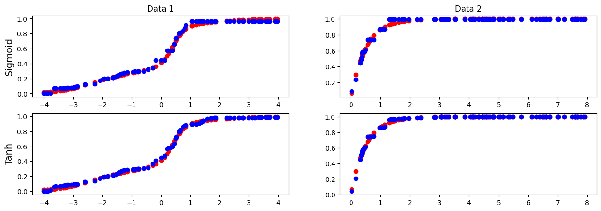
각 모델이 bounded 조건을 잘 만족하는지 역시 확인할 수 있다.
# bounded 검증
print(torch.all((0 <= test_pred_sig1) & (test_pred_sig1 <= 1)))
print(torch.all((0 <= test_pred_sig2) & (test_pred_sig2 <= 1)))
print(torch.all((0 <= test_pred_tanh1) & (test_pred_tanh1 <= 1)))
print(torch.all((0 <= test_pred_tanh2) & (test_pred_tanh2 <= 1)))
3. Origin-Passing Monotone Neural Network
원점()을 지나도록 하기 위해 다음 세 가지 기법을 소개하고 효용성을 비교할 것이다.
- 모든 bias 제거
- 마지막 layer에서 bias 제거
- 원점을 지나는 증가함수 곱하기
세 방법 모두 단조성(증가)을 해치지 않으면서 원점을 지남을 어렵지 않게 확인할 수 있다. 단, 세 번째 방법은 양수 정의역에서만 사용할 수 있다. 이후 실험을 진행할 때 세 번째 방법은 양수 영역에서 sampling한 데이터를 사용할 것이다.
우선 Monotonic Dense Block을 가져오자.
import torch
import torch.nn as nn
import torch.nn.functional as F
from torch.nn.parameter import Parameter
from torch.nn.modules.module import Module

import numpy as np
import matplotlib.pyplot as plt

# MonoBlock 구현
## activation : relu, elu, selu, none 중 선택
class MonoBlock(Module):
    def __init__(self, in_feature:int, out_feature:int, mono_indicator = 'inc', activation = 'none', activation_partition = (0,0,1)):
        super().__init__()
        self.activation = activation
        self.activation_partition = activation_partition

        self.in_feature = in_feature
        self.out_feature = out_feature
        self.mono_indicator = mono_indicator

        self.W = Parameter(torch.randn(self.in_feature, self.out_feature))
        self.b = Parameter(torch.randn(self.out_feature))

    def get_activation(self):
        convex = getattr(F, self.activation)
        def concave(x):
            return -convex(-x)
        def saturated(x):
            plus = -convex(-x+torch.ones_like(x)) + convex(torch.ones_like(x))
            minus = convex(x+torch.ones_like(x)) - convex(torch.ones_like(x))
            return torch.where(x >= 0, plus, minus)
        return convex, concave, saturated

    def activation_index(self, x):
        if sum(self.activation_partition) != 1:
            raise ValueError(f"sum of activation_partition must be 1")
        if len(self.activation_partition) != 3:
            raise ValueError(f"length of activation_partition must be 3")

        convex_num = int(self.activation_partition[0] * len(x.T))
        concave_num = int(self.activation_partition[1] * len(x.T))
        return convex_num, convex_num+concave_num, len(x.T)

    def forward(self, x):
        if len(x.shape) == 1:
            x = x.reshape(-1, 1)
        if self.mono_indicator == 'inc':
            self.mono_indicator = torch.ones(x.shape[1])
        if x.shape[1] != self.in_feature:
            raise ValueError(f"matrix multiplication cannot be implemented : {x.shape[0]}x{x.shape[1]} and {self.in_feature}x{self.out_feature}")
        if len(self.mono_indicator) != self.in_feature:
            raise ValueError(f"number of variable does not match : {len(self.mono_indicator)} and {self.in_feature}")

        mono_oper = torch.tensor(self.mono_indicator).reshape(-1, 1) * torch.abs(self.W)
        W_oper = torch.where(torch.abs(mono_oper) >= torch.abs(self.W), mono_oper, self.W)
        x = torch.matmul(x, W_oper) + self.b

        convex_idx, concave_idx, saturated_idx = self.activation_index(x)
        if self.activation == 'none':
            out = torch.cat([x.T[:convex_idx], x.T[convex_idx:concave_idx], x.T[concave_idx:saturated_idx]], dim=0)
        else:
            convex_act, concave_act, saturated_act = self.get_activation()
            out = torch.cat([convex_act(x.T[:convex_idx]), concave_act(x.T[convex_idx:concave_idx]), saturated_act(x.T[concave_idx:saturated_idx])], dim=0).T

        return out
모든 bias 제거
모든 bias의 requiredgrad를 False로 설정하고 초기값을 0으로 설정한다.
# 전체 bias 제거 - 학습X, 0 부여
class MonoNet(nn.Module):
    def __init__(self):
        super().__init__()
        self.mono = nn.Sequential(
            MonoBlock(1, 32, mono_indicator=[1], activation='elu', activation_partition=(0, 0, 1)),
            MonoBlock(32, 24, activation='elu', activation_partition=(0, 0, 1)),
            MonoBlock(24, 16, activation='elu', activation_partition=(0, 0, 1)),
            MonoBlock(16, 8, activation='elu', activation_partition=(0, 0, 1)),
            MonoBlock(8, 1)
        )

    def forward(self, x):
        return self.mono(x)

model_nobias1 = MonoNet()
model_nobias2 = MonoNet()

def init_weights(m):
    if isinstance(m, MonoBlock):
        m.b.data.fill_(0)
        m.b.requires_grad_(False)

model_nobias1.apply(init_weights)
model_nobias2.apply(init_weights)
마지막 layer에서 bias 제거
마지막 layer를 거친 후, 최종 bias를 빼는 origin 메소드를 적용시킨다.
# 마지막 layer에서 bias 제거
class MonoNet_mbias(nn.Module):
    def __init__(self):
        super().__init__()
        self.mono = nn.Sequential(
            MonoBlock(1, 32, mono_indicator=[1], activation='elu', activation_partition=(0, 0, 1)),
            MonoBlock(32, 24, activation='elu', activation_partition=(0, 0, 1)),
            MonoBlock(24, 16, activation='elu', activation_partition=(0, 0, 1)),
            MonoBlock(16, 8, activation='elu', activation_partition=(0, 0, 1)),
            MonoBlock(8, 1)
        )

    def origin(self, x):
        zero = torch.zeros_like(x)
        return self.mono(zero)

    def forward(self, x):
        return self.mono(x) - self.origin(x)

model_mbias1 = MonoNet_mbias()
model_mbias2 = MonoNet_mbias()
원점을 지나는 증가함수 곱하기
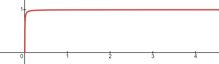
원점을 지나는 함수를 곱하여 강제로 원점을 지나도록 한다. 이때 단조성(증가)을 유지하기 위해 곱해지는 함수 역시 증가함수로 설정하며, 학습에 미치는 영향을 가능한 줄이기 위해 원점 이외에선 상수함수에 가까운 함수를 선택한다.
다만 이는 0 이상의 정의역에서만 사용할 수 있다. 만약 음수 영역에서도 함수를 정의하려면, 단조성을 지키기 위해 함수값이 음수가 될 수 밖에 없고 이는 학습에 적지 않은 영향을 준다.
또한 함수의 합성과는 달리, 함숫값이 항상 양수인 증가함수를 곱한 것이 증가함수이기 위해선 원래 함수 역시 함숫값이 항상 양수인 증가함수여야 한다. 이를 위해 마지막 layer를 통과한 값에 다음 함수를 우선 합성한다.
7주차 주제인 Dynamic Pricing은 항상 0 이상의 정의역에서만 다루어지는 문제이므로 세 번째 방법 역시 사용이 가능하다.
# 원점을 지나는 증가함수 곱하기 (양수에서만 정의)
class MonoNet_mul(nn.Module):
    def __init__(self):
        super().__init__()
        self.mono = nn.Sequential(
            MonoBlock(1, 32, mono_indicator=[1], activation='elu', activation_partition=(0, 0, 1)),
            MonoBlock(32, 24, activation='elu', activation_partition=(0, 0, 1)),
            MonoBlock(24, 16, activation='elu', activation_partition=(0, 0, 1)),
            MonoBlock(16, 8, activation='elu', activation_partition=(0, 0, 1)),
            MonoBlock(8, 1)
        )

    def origin(self, x):
        if torch.any(x.T < 0):
            raise ValueError(f"input value 'x' should be non-negative")
        return torch.log(3*x.T+1) / (0.01 + torch.log(3*x.T+1))

    def forward(self, x):
        out = self.mono(x)
        return torch.where(out>=1, out, torch.exp(out-1)) * self.origin(x)


model_mul1 = MonoNet_mul()
model_mul2 = MonoNet_mul()
모델 검증
검증에 사용할 train, valid, test 데이터를 생성한다. 입력/출력이 모두 1차원인 다음 두 모의함수를 사용할 것이다.
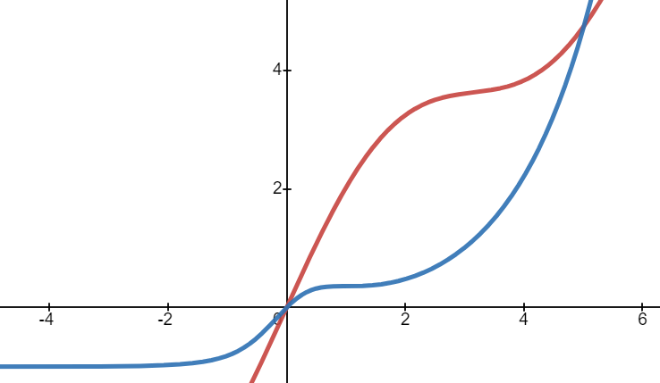
- 붉은 그래프 :
- 푸른 그래프 :
# Reproduce를 위한 seed 고정
random_seed = 42
torch.manual_seed(random_seed)
np.random.seed(random_seed)

# 데이터 생성 _ train, valid, test
def data_generate(num_sample, noise):
    X = np.random.uniform(-4, 4, num_sample)
    Y1 = np.log(X/5 + 1) + X + np.sin(X) + noise * np.random.normal(0, 1, num_sample)
    Y2 = np.exp(X) / (X**2 + 1) - 1 + noise * np.random.normal(0, 1, num_sample)
    return torch.tensor(X, dtype=torch.float), torch.tensor(Y1, dtype=torch.float), torch.tensor(Y2, dtype=torch.float)

def data_generate_pos(num_sample, noise):
    X = np.random.uniform(0, 8, num_sample)
    Y1 = np.log(X/5 + 1) + X + np.sin(X) + noise * np.random.normal(0, 1, num_sample)
    Y2 = np.exp(X) / (X**2 + 1) - 1 + noise * np.random.normal(0, 1, num_sample)
    return torch.tensor(X, dtype=torch.float), torch.tensor(Y1, dtype=torch.float), torch.tensor(Y2, dtype=torch.float)

train_x, train_y1, train_y2 = data_generate(800, 0.1)
valid_x, valid_y1, valid_y2 = data_generate(100, 0.1)
test_x, test_y1, test_y2 = data_generate(100, 0.1)

train_xp, train_yp1, train_yp2 = data_generate_pos(800, 0.1)
valid_xp, valid_yp1, valid_yp2 = data_generate_pos(100, 0.1)
test_xp, test_yp1, test_yp2 = data_generate_pos(100, 0.1)
두 데이터에 대해, 세 모델에 각각 학습시킨다.
# 모델학습
## model_nobias
my_param_nobias = {'learning_rate' : 0.001,
                   'num_epoch' : 10000}

## 1번 데이터
criterion = nn.MSELoss()
optimizer = torch.optim.Adam(model_nobias1.parameters(), lr=my_param_nobias['learning_rate'])
best_valid_loss_torch = 10**9

for epoch in range(1, my_param_nobias['num_epoch']+1):
    model_nobias1.train()

    output = model_nobias1(train_x)
    train_loss = criterion(output, train_y1)

    optimizer.zero_grad()
    train_loss.backward()
    optimizer.step()

    with torch.no_grad():
        model_nobias1.eval()
        if epoch % 500 == 0:
            valid_output = model_nobias1(valid_x)
            valid_loss = criterion(valid_output, valid_y1)
            print(f"    [Epoch {epoch}] Valid loss : {valid_loss}")

            if best_valid_loss_torch > valid_loss:
                best_valid_loss_torch = valid_loss

print(f"[PyTorch] Best valid loss : {best_valid_loss_torch}")


## 2번 데이터
criterion = nn.MSELoss()
optimizer = torch.optim.Adam(model_nobias2.parameters(), lr=my_param_nobias['learning_rate'])
best_valid_loss_torch = 10**9

for epoch in range(1, my_param_nobias['num_epoch']+1):
    model_nobias2.train()

    output = model_nobias2(train_x)
    train_loss = criterion(output, train_y2)

    optimizer.zero_grad()
    train_loss.backward()
    optimizer.step()

    with torch.no_grad():
        model_nobias2.eval()
        if epoch % 500 == 0:
            valid_output = model_nobias2(valid_x)
            valid_loss = criterion(valid_output, valid_y2)
            print(f"    [Epoch {epoch}] Valid loss : {valid_loss}")

            if best_valid_loss_torch > valid_loss:
                best_valid_loss_torch = valid_loss

print(f"[PyTorch] Best valid loss : {best_valid_loss_torch}")
# 모델학습
## model_mbias
my_param_mbias = {'learning_rate' : 0.001,
'num_epoch' : 10000}
## 1번 데이터
criterion = nn.MSELoss()
optimizer = torch.optim.Adam(model_mbias1.parameters(), lr=my_param_mbias['learning_rate'])
best_valid_loss_torch = 10**9
for epoch in range(1, my_param_mbias['num_epoch']+1):
model_mbias1.train()
output = model_mbias1(train_x)
train_loss = criterion(output, train_y1)
optimizer.zero_grad()
train_loss.backward()
optimizer.step()
with torch.no_grad():
model_mbias1.eval()
if epoch % 500 == 0:
valid_output = model_mbias1(valid_x)
valid_loss = criterion(valid_output, valid_y1)
print(f" [Epoch {epoch}] Valid loss : {valid_loss}")
if best_valid_loss_torch > valid_loss:
best_valid_loss_torch = valid_loss
print(f"[PyTorch] Best valid loss : {best_valid_loss_torch}")
## 2번 데이터
criterion = nn.MSELoss()
optimizer = torch.optim.Adam(model_mbias2.parameters(), lr=my_param_mbias['learning_rate'])
best_valid_loss_torch = 10**9
for epoch in range(1, my_param_mbias['num_epoch']+1):
model_mbias2.train()
output = model_mbias2(train_x)
train_loss = criterion(output, train_y2)
optimizer.zero_grad()
train_loss.backward()
optimizer.step()
with torch.no_grad():
model_mbias2.eval()
if epoch % 500 == 0:
valid_output = model_mbias2(valid_x)
valid_loss = criterion(valid_output, valid_y2)
print(f" [Epoch {epoch}] Valid loss : {valid_loss}")
if best_valid_loss_torch > valid_loss:
best_valid_loss_torch = valid_loss
print(f"[PyTorch] Best valid loss : {best_valid_loss_torch}")# 모델학습
## model_mul
my_param_mul = {'learning_rate' : 0.001,
'num_epoch' : 10000}
## 1번 데이터
criterion = nn.MSELoss()
optimizer = torch.optim.Adam(model_mul1.parameters(), lr=my_param_mul['learning_rate'])
best_valid_loss_torch = 10**9
for epoch in range(1, my_param_mul['num_epoch']+1):
model_mul1.train()
output = model_mul1(train_xp)
train_loss = criterion(output, train_yp1)
optimizer.zero_grad()
train_loss.backward()
optimizer.step()
with torch.no_grad():
model_mul1.eval()
if epoch % 500 == 0:
valid_output = model_mul1(valid_xp)
valid_loss = criterion(valid_output, valid_yp1)
print(f" [Epoch {epoch}] Valid loss : {valid_loss}")
if best_valid_loss_torch > valid_loss:
best_valid_loss_torch = valid_loss
print(f"[PyTorch] Best valid loss : {best_valid_loss_torch}")
## 2번 데이터
criterion = nn.MSELoss()
optimizer = torch.optim.Adam(model_mul2.parameters(), lr=my_param_mul['learning_rate'])
best_valid_loss_torch = 10**9
for epoch in range(1, my_param_mul['num_epoch']+1):
model_mul2.train()
output = model_mul2(train_xp)
train_loss = criterion(output, train_yp2)
optimizer.zero_grad()
train_loss.backward()
optimizer.step()
with torch.no_grad():
model_mul2.eval()
if epoch % 500 == 0:
valid_output = model_mul2(valid_xp)
valid_loss = criterion(valid_output, valid_yp2)
print(f" [Epoch {epoch}] Valid loss : {valid_loss}")
if best_valid_loss_torch > valid_loss:
best_valid_loss_torch = valid_loss
print(f"[PyTorch] Best valid loss : {best_valid_loss_torch}")test data에 대해 각 모델의 예측 결과는 다음과 같다.
# BddMonoNet_Sig, BddMonoNet_Tanh 모델 평가
test_pred_nobias1 = model_nobias1(test_x)
test_pred_nobias2 = model_nobias2(test_x)
test_pred_mbias1 = model_mbias1(test_x)
test_pred_mbias2 = model_mbias2(test_x)
test_pred_mul1 = model_mul1(test_xp)
test_pred_mul2 = model_mul2(test_xp)


# 결과 시각화
fig_ori_test = plt.figure()
fig_ori_test.set_figwidth(15)
fig_ori_test.set_figheight(10)


ax_ori_test_nobias1 = fig_ori_test.add_subplot(321)
ax_ori_test_nobias1.scatter(test_x.detach(), test_y1.detach(), color='r')
ax_ori_test_nobias1.scatter(test_x.detach(), test_pred_nobias1.detach(), color='b')

ax_ori_test_nobias2 = fig_ori_test.add_subplot(322)
ax_ori_test_nobias2.scatter(test_x.detach(), test_y2.detach(), color='r')
ax_ori_test_nobias2.scatter(test_x.detach(), test_pred_nobias2.detach(), color='b')

ax_ori_test_mbias1 = fig_ori_test.add_subplot(323)
ax_ori_test_mbias1.scatter(test_x.detach(), test_y1.detach(), color='r')
ax_ori_test_mbias1.scatter(test_x.detach(), test_pred_mbias1.detach(), color='b')

ax_ori_test_mbias2 = fig_ori_test.add_subplot(324)
ax_ori_test_mbias2.scatter(test_x.detach(), test_y2.detach(), color='r')
ax_ori_test_mbias2.scatter(test_x.detach(), test_pred_mbias2.detach(), color='b')

ax_ori_test_mul1 = fig_ori_test.add_subplot(325)
ax_ori_test_mul1.scatter(test_xp.detach(), test_yp1.detach(), color='r')
ax_ori_test_mul1.scatter(test_xp.detach(), test_pred_mul1.detach(), color='b')

ax_ori_test_mul2 = fig_ori_test.add_subplot(326)
ax_ori_test_mul2.scatter(test_xp.detach(), test_yp2.detach(), color='r')
ax_ori_test_mul2.scatter(test_xp.detach(), test_pred_mul2.detach(), color='b')


ax_ori_test_nobias1.set_title('Data 1')
ax_ori_test_nobias2.set_title('Data 2')
ax_ori_test_nobias1.set_ylabel('No bias', fontsize=14)
ax_ori_test_mbias1.set_ylabel('Minus bias', fontsize=14)
ax_ori_test_mul1.set_ylabel('Multiple', fontsize=14)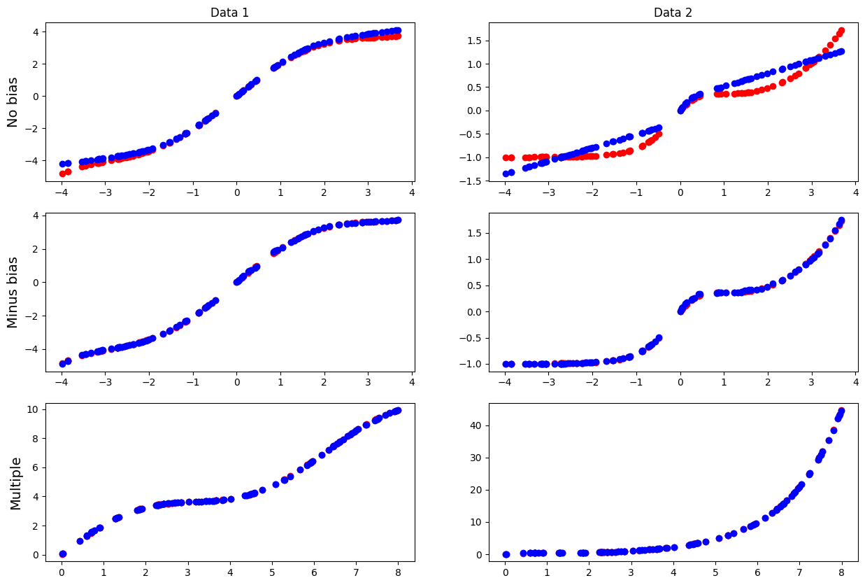
- 모든 bias를 제거한 모델은 다른 모델에 비해 표현력이 떨어졌고, 그 결과 복잡한 함수를 비교적 간단한 모형으로 예측함을 확인할 수 있다.
- 마지막 layer에서 bias를 제거한 모델은 마지막 bias에 의해 전체 bias가 영향을 받는다. 만약 원점 주변 데이터를 학습하지 못한다면 편향된 bias가 나타날 것이고, 이는 전체 모델의 편향을 발생시킬 것이다.
- 증가함수를 곱하는 모델은 정의역이 0 이상으로 제한되며 0 주변에서 왜곡이 발생할 가능성이 있다. 하지만 전체적인 bias는 두 번째 방법보다 낮을 것으로 예상된다.
각 모델이 원점을 잘 지나는지 역시 확인할 수 있다.
# 원점 통과 검증
print(model_nobias2(torch.tensor([0], dtype=torch.float)) == torch.tensor([0]))
print(model_mbias1(torch.tensor([0], dtype=torch.float)) == torch.tensor([0]))
print(model_mul1(torch.tensor([0], dtype=torch.float)) == torch.tensor([0]))