관련논문
- Cox, Cox-Regression Models and Life Tables
- Choi Y, Semi-Parametric Contextual Pricing Algorithm using Cox Proportional
Hazards Model
참고교재
- Wooldridge (2010), Econometric Analysis of Cross Section and Panel Data, 2nd Edition, MIT Press.
1. Introduction
상품이나 서비스를 판매하는 입장에서 판매 가격을 결정하는 것은 상당히 중요한 문제다. 판매자는 최대 판매수익을 얻을 수 있는 가격을 설정할 것이며, 이를 위해선 고객의 지불의사가격(WTP, Willing To Pay)을 아는 것이 중요하다.
하지만 WTP는 고객마다 다르며 판매자가 이를 알 방법 또한 없다. 하지만 과거의 판매 기록 데이터를 기반으로 고객의 WTP 분포를 추정할 수 있다면, 고객 별로 가격을 달리 책정하는 Contextual Dynamic Pricing 전략을 활용할 수 있을 것이다.
판매 데이터의 가장 큰 특징은 type-I interval censored data라는 점이다. 예를 들어 커피 한 잔을 1500원에 판매했다면 고객이 생각하는 커피 한 잔의 WTP는 1500원보다 높을 것이며, 생각했던 가격보다 저렴하게 판매하기 때문에 구매했다고 추측할 수 있다. 결국 고객의 WTP는 하나의 값이 아닌 구간(interval)으로 나타나게 된다.
이러한 데이터로부터 확률분포를 추정하기 위해 앞서 비모수적 추정에 대해 알아보았다. 이번에는 고객의 정보를 고려할 것이므로 Contextual vector 가 등장할 것이며, 각 정보가 가격 결정에 미치는 정도를 살펴볼 것이다. 이를 위해 Cox Proportional Hazard Model을 사용한다.
2. Cox Proportional Hazard Model
Cox PH 모델은 생존분석의 기법 중 하나이다. 우리가 관심있어하는 부분은, '특정 사건이 언제 발생하는가'인데, 단 한 번만 발생하는 사건(죽음, 실패 등)을 다루므로 충분히 생존분석이라 말할 수 있겠다. 생존-죽음을 넓은 의미로 보면 재직-해고, 건강-발병 등에 대입할 수 있다.
실패 시점을 나타내는 확률변수 의 누적분포함수 는
로 정의되며, 시간 이내에 실패할 확률을 의미한다. 이와는 반대로 시점까지 생존할 확률을 나타내는 생존함수(survivor function) 는
로 나타낸다.
일반적으로 시간의 흐름에 따라 생존 죽음 상태로 이어지는데, 시점에서 죽음이 발생할 가능성(=생존을 벗어날 가능성)을 나타내는 위험함수(hazard function) 는
로 나타내며, 결국 는
와 같이 에 의해 결정된다고 볼 수 있다. 만약 (상수함수)라면 는 모수가 인 지수분포를 따르게 된다.
현실적으로 생각해보면 개개인마다의 생존함수는 모두 다를 것이다. 이를 공변량(covariates) 로 표현할 것이며, 이에 따른 위험함수 는
로 나타낸다. 는 치역이 양수인 함수이며, 는 baseline hazard function으로, covariate에 관계없이 에 공통적으로 포함된 함수이다.
일반적으로 로 나타낸다. 즉, covariate vector 의 각 변수가 분포함수에 얼마나 영향을 미치는지를 나타내는 가중치 벡터 로 해석할 수 있고, 는 일 때를 의미하게 된다.
covariate 가 전제되었을 때의 생존함수 는
로 나타난다. 는 와 마찬가지로 covariate에 관계없는() baseline function과 같으며, 앞으로 로 표기할 것이다.
3. Contextual Pricing using Cox PH Model
어떤 물건을 구매하는데 있어 고객이 생각하는 WTP를 라 하고, 판매자가 제시하는 물건의 가격을 라 하자. 구매자의 정보를 라 하고, 물건 구매 여부를 라 하자. 물건을 구매했다면 , 구매하지 않았다면 인 것이다.
예를 들어 고객이 비행기 티켓을 구매하는 상황을 생각해볼 수 있다. 항공사는 비행기 티켓 가격을 에 제시하고, 구매자는 마음속으로 의 가격을 생각하며 판매가격이 이하라면 티켓을 구매할 것이다. 구매자의 정보 는 나이, 성별, 거주지, 행선지 등을 포함할 것이다. 즉
이다.
판매자는 의 분포를 알고싶을 것이다. 이를 확률변수로 두고 '구매'를 생존, '구매하지 않음'을 죽음으로 정의한다면
와 같다. 여기서
는 Cumulative hazard function이라 불린다.
이러한 type-I interval censored data로부터 의 분포를 추정하자. 위 정의에 의해
이므로 (혹은 )를 추정하기 위한 MLE는
이다. 이때 는 sample의 개수이다.
4. Contextual Pricing Neural Network
지금까지의 내용을 Neural Network로 구현해보자. Neural Network로 추정해야 할 것은 와 가 될 것이다. 가 주어진다는 점을 생각해보면 는 parametric한 추정이며, 는 Non-parametric한 추정이고, 결국 둘 모두를 고려하는 Semi-parametric 추정인 것이다.
현실적으로 우리가 알 수 있는 데이터는 이고, 이로부터 알려지지 않은 의 분포를 추정해야 한다. 이러한 데이터는 Neural Network로 하여금 가 아닌 를 직접 학습시킨다.
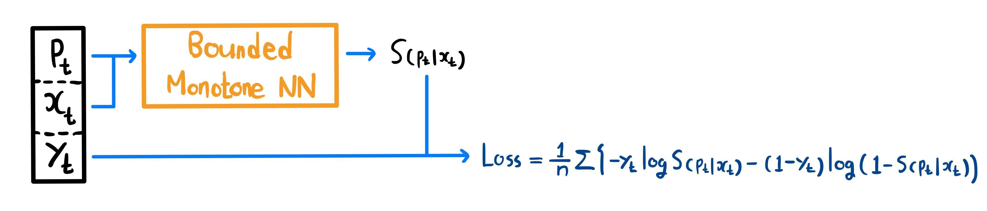
따라서 의 각 변수가 의 분포에 어떤 영향을 끼치는지 궁금하지 않다면, 위 구조로 네트워크를 학습시키면 된다.
만약 까지 추정하고자 한다면 다음과 같이 를 학습하는 과 를 학습하는 를 구성하여 합하는 방법을 제안한다.
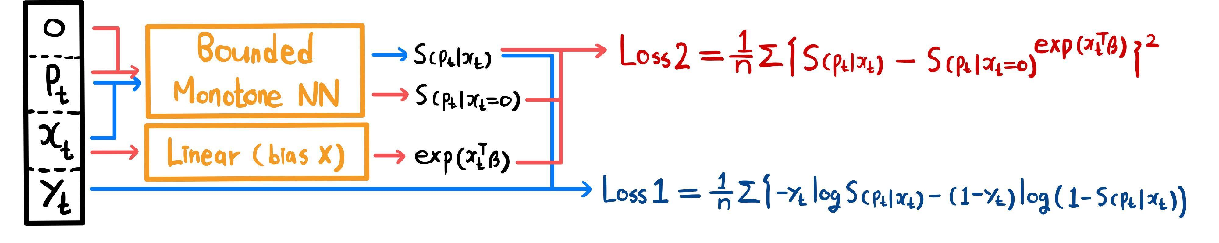
- 은 첫 번째 네트워크 구조와 같은 것으로, 를 학습하도록 한다.
- 는 를 학습하도록 한다.
- 각 마다 는 모두 다르지만, 를 공통으로 갖는다는 성질이 있다.
- 공통으로 갖는 가 과 같아지도록 학습함으로써 속의 가 자동으로 결정되도록 한다.
같은 방법으로 를 추정하도록 설계할 수 있다. 이므로 비슷한 결과를 얻을 수 있다.
실험1. 단일차원 Contextual
- True
- 초기
- True
랜덤시드를 고정하고 데이터를 생성한다.
import torch
import torch.nn as nn
import torch.nn.functional as F
from torch.nn.parameter import Parameter
from torch.nn.modules.module import Module
import numpy as np
import scipy.stats as st
import matplotlib.pyplot as plt
# Seed 고정 함수
def RandomFix(random_seed):
torch.manual_seed(random_seed)
torch.cuda.manual_seed(random_seed)
np.random.seed(random_seed)
device = torch.device("cuda" if torch.cuda.is_available() else "cpu")
print(device)
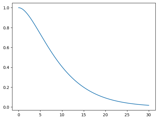
# 추정하고자 하는 beta : -2
# 추정하고자 하는 F: 감마분포(alpha=2, beta=0.2)
class RV_Sampler(st.rv_continuous):
def __init__(self, cox):
super().__init__()
self.cox = cox
def _cdf(self, x):
return 1 - (st.gamma.sf(x=x, a=2, loc=0, scale=5))**self.cox
def generate_dataC(num_sample):
beta = np.array([-2])
x_t = np.random.randn(len(beta), num_sample)
cox_t = np.exp(np.dot(beta, x_t))
v_t = np.array([RV_Sampler(cox=val).rvs(size=1)[0] for val in cox_t])
p_t = st.uniform.rvs(size=num_sample) * 30
y_t = (v_t >= p_t).astype(int)
return torch.tensor(x_t.T, dtype=torch.float), torch.tensor(p_t, dtype=torch.float), torch.tensor(y_t, dtype=torch.float)- 확률분포에서 샘플링하는 방법으로 scipy.stats의 rvs를 이용하였다. 이는 에서 샘플링한 값에 cdf의 역함수를 씌우는 Inverse CDF Method를 사용한다.
- 의 그래프는 다음과 같다.
모델 구성은 다음과 같다. 이전에 구현한 MonoBlock을 바탕으로 MonoNet_bdd( 추정), MonoNet_mul( 추정)을 구성하였다.
class MonoBlock(Module):
    def __init__(self, in_feature:int, out_feature:int, mono_indicator = 'inc', activation = 'none', activation_partition = (0,0,1)):
        super().__init__()
        self.activation = activation
        self.activation_partition = activation_partition

        self.in_feature = in_feature
        self.out_feature = out_feature
        self.mono_indicator = mono_indicator

        self.W = Parameter(torch.randn(self.in_feature, self.out_feature))
        self.b = Parameter(torch.randn(self.out_feature))

    def get_activation(self):
        convex = getattr(F, self.activation)
        def concave(x):
            return -convex(-x)
        def saturated(x):
            plus = -convex(-x+torch.ones_like(x)) + convex(torch.ones_like(x))
            minus = convex(x+torch.ones_like(x)) - convex(torch.ones_like(x))
            return torch.where(x >= 0, plus, minus)
        return convex, concave, saturated

    def activation_index(self, x):
        if sum(self.activation_partition) != 1:
            raise ValueError(f"sum of activation_partition must be 1")
        if len(self.activation_partition) != 3:
            raise ValueError(f"length of activation_partition must be 3")

        convex_num = int(self.activation_partition[0] * len(x.T))
        concave_num = int(self.activation_partition[1] * len(x.T))
        return convex_num, convex_num+concave_num, len(x.T)

    def forward(self, x):
        if len(x.shape) == 1:
            x = x.reshape(-1, 1)
        if self.mono_indicator == 'inc':
            self.mono_indicator = torch.ones(x.shape[1])
        if x.shape[1] != self.in_feature:
            raise ValueError(f"matrix multiplication cannot be implemented : {x.shape[0]}x{x.shape[1]} and {self.in_feature}x{self.out_feature}")
        if len(self.mono_indicator) != self.in_feature:
            raise ValueError(f"number of variable does not match : {len(self.mono_indicator)} and {self.in_feature}")

        mono_oper = torch.tensor(self.mono_indicator).to(device).reshape(-1, 1) * torch.abs(self.W)
        W_oper = torch.where(torch.abs(mono_oper) >= torch.abs(self.W), mono_oper, self.W)
        x = torch.matmul(x, W_oper) + self.b

        convex_idx, concave_idx, saturated_idx = self.activation_index(x)
        if self.activation == 'none':
            out = torch.cat([x.T[:convex_idx], x.T[convex_idx:concave_idx], x.T[concave_idx:saturated_idx]], dim=0).T
        else:
            convex_act, concave_act, saturated_act = self.get_activation()
            out = torch.cat([convex_act(x.T[:convex_idx]), concave_act(x.T[convex_idx:concave_idx]), saturated_act(x.T[concave_idx:saturated_idx])], dim=0).T

        return out


class MonoNet_bdd(nn.Module):
    def __init__(self, context_size):
        super().__init__()
        self.context_size = context_size
        self.linear = nn.Linear(self.context_size, 1, bias=False)
        self.mono = nn.Sequential(
            MonoBlock(2, 32, mono_indicator=[0, -1], activation='elu', activation_partition=(0, 0, 1)),
            MonoBlock(32, 16, activation='elu', activation_partition=(0, 0, 1)),
            MonoBlock(16, 8, activation='elu', activation_partition=(0, 0, 1)),
            MonoBlock(8, 1)
        )

        eps = 1e-6
        for m in self.modules():
            if isinstance(m, MonoBlock):
                torch.nn.init.uniform_(m.W)
                torch.nn.init.uniform_(m.b, a=-1, b=1)
            elif isinstance(m, nn.Linear):
                torch.nn.init.uniform_(m.weight, a=-1, b=1)


    def coxfunc(self, x):
        return torch.exp(self.linear(x))

    def forward(self, x, p):
        cat = torch.cat([x, p.reshape(-1, 1)], dim=1)
        S_x = torch.sigmoid(self.mono(cat))

        cox = self.coxfunc(x)
        S_0 = S_x**(1/cox)

        return S_x, S_0, cox


class MonoNet_mul(nn.Module):
    def __init__(self, context_size):
        super().__init__()
        self.context_size = context_size
        self.linear = nn.Linear(self.context_size, 1, bias=False)
        self.mono = nn.Sequential(
            MonoBlock(2, 32, mono_indicator=[0, 1], activation='elu', activation_partition=(0, 0, 1)),
            MonoBlock(32, 16, activation='elu', activation_partition=(0, 0, 1)),
            MonoBlock(16, 8, activation='elu', activation_partition=(0, 0, 1)),
            MonoBlock(8, 1)
        )

        eps = 1e-6
        for m in self.modules():
            if isinstance(m, MonoBlock):
                torch.nn.init.uniform_(m.W)
                torch.nn.init.uniform_(m.b, a=-1, b=1)
            elif isinstance(m, nn.Linear):
                torch.nn.init.uniform_(m.weight, a=-1, b=1)


    def coxfunc(self, x):
        return torch.exp(self.linear(x))

    def origin(self, x):
        result = torch.log(3*x+1) / (0.01 + torch.log(3*x+1))
        return result.reshape(-1, 1)

    def forward(self, x, p):
        cat = torch.cat([x, p.reshape(-1, 1)], dim=1)
        out = self.mono(cat)
        L_x = torch.where(out>=1, out, torch.exp(out-1)) * self.origin(p)

        cox = self.coxfunc(x)
        L_0 = L_x / cox

        return L_x, L_0, cox
학습에 사용될 공통 하이퍼파라미터를 정의하였다.
common_param = {'learning_rate' : 0.01,
                'num_epoch' : 5000}
num_repl = 100
데이터를 생성하고 모델을 학습시킨다.
# 모델학습 _ S추정 _ replication
y_rate_SC = []
S_errorC = []
S_betaC_x = [0]
S_betaC_y = []
S_betaC_res = []

p = np.linspace(0.1, 30, 200)
P = torch.tensor(p, dtype=torch.float).reshape(-1, 1).to(device)
X = torch.zeros((200, 1), dtype=torch.float).to(device)
baseX = torch.zeros((10000, 1), dtype=torch.float).to(device)
gtC = st.gamma.cdf(p, a=2, loc=0, scale=5).reshape(-1, 1)

for idx in range(1, num_repl+1):
    RandomFix(idx)
    print(f"====={idx} Replication =====")

    modelS = MonoNet_bdd(1)
    modelS.to(device)
    optimizer = torch.optim.Adam(modelS.parameters(), lr=common_param['learning_rate'])

    if idx == 1:
        for m in modelS.modules():
            if isinstance(m, nn.Linear):
                S_betaC_y.append(m.weight[0].cpu().detach().numpy()[0])

    train_x, train_p, train_y = generate_dataC(10000)
    y_rate_SC.append(sum(train_y) / 10000)

    train_x = train_x.to(device)
    train_p = train_p.to(device)
    train_y = train_y.reshape(-1, 1).to(device)

    for epoch in range(1, common_param['num_epoch']+1):
        modelS.train()

        S_x, S_0, cox = modelS(train_x, train_p)
        S_00 = modelS(baseX, train_p)[0]

        loss1 = torch.mean(-1 * train_y * torch.log(S_x) - (1-train_y) * torch.log(1 - S_x))
        loss2 = torch.mean((S_00**cox - S_x)**2)
        train_loss = loss1 + loss2
        if epoch % 100 == 0:
            print(f"  [Epoch {epoch}] Train loss : {train_loss}")

        optimizer.zero_grad()
        train_loss.backward()
        optimizer.step()

        if idx == 1:
            for m in modelS.modules():
                if isinstance(m, nn.Linear):
                    cand = m.weight[0].cpu().detach().numpy()[0]
                    if S_betaC_y[-1] != cand:
                        S_betaC_x.append(epoch)
                        S_betaC_y.append(cand)
    for m in modelS.modules():
        if isinstance(m, nn.Linear):
            S_betaC_res.append(m.weight[0].cpu().detach().numpy()[0])

    F_0 = 1 - modelS(X, P)[1]
    S_errorC.append(gtC - F_0.cpu().detach().numpy())

fig = plt.figure()
fig.set_figwidth(20)

ax1 = fig.add_subplot(131)
ax1.plot(p, gtC, 'r')
ax1.plot(p, -1 * sum(S_errorC)/len(S_errorC) + gtC, color='b')

ax2 = fig.add_subplot(132)
ax2.plot(S_betaC_x, S_betaC_y)

ax3 = fig.add_subplot(133)
ax3.hist(S_betaC_res, bins=100)

print(f"y_t=1 비율 : {sum(y_rate_SC).numpy()/len(y_rate_SC)}")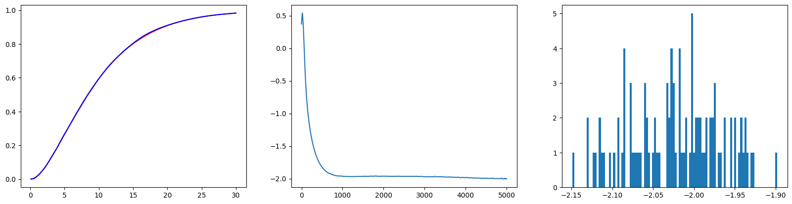
print(f"Std(RMSE) : {np.sqrt(np.mean(sum(val**2 for val in S_errorC)))}")- 우연에 의존한 결과가 아님을 보이기 위해 같은 실험을 Random seed 값만 달리하여 100번 진행하였다(Replication). 그 결과 와 모두 잘 추정하는 모습을 볼 수 있었다.
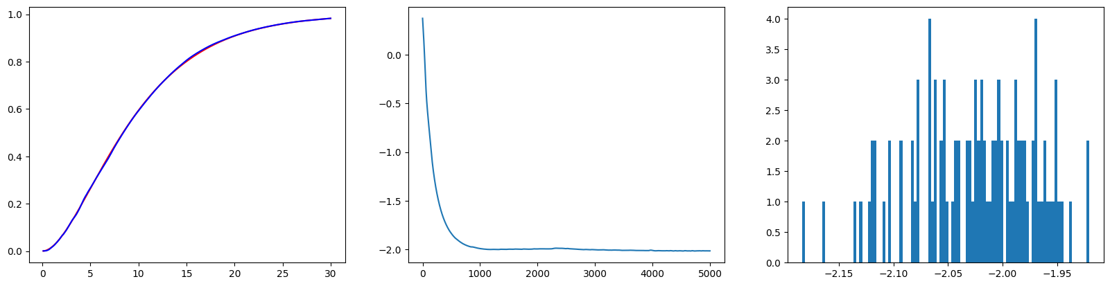
- 첫 번째 그래프는 100번의 Replication으로부터 도출된 의 평균값을 그린 그래프이다.
- 붉은 색은 True 이며, 푸른 색은 추정한 이다.
- 두 번째 그래프는 첫 번째 Replication에서 값의 변화를 나타낸 그래프다.
- 세 번째 그래프는 100번의 Replication동안 나타난 의 히스토그램이다. 대체로 True 값인 근처에 잘 모인 모습이다.
같은 방법으로 를 추정하는 과정이다.
# 모델학습 _ L추정 _ replication
y_rate_LC = []
L_errorC = []
L_betaC_x = [0]
L_betaC_y = []
L_betaC_res = []

p = np.linspace(0.1, 30, 200)
P = torch.tensor(p, dtype=torch.float).reshape(-1, 1).to(device)
X = torch.zeros((200, 1), dtype=torch.float).to(device)
baseX = torch.zeros((10000, 1), dtype=torch.float).to(device)
gtC = st.gamma.cdf(p, a=2, loc=0, scale=5).reshape(-1, 1)

for idx in range(1, num_repl+1):
    RandomFix(idx)
    print(f"====={idx} Replication =====")

    modelL = MonoNet_mul(1)
    modelL.to(device)
    optimizer = torch.optim.Adam(modelL.parameters(), lr=common_param['learning_rate'])

    if idx == 1:
        for m in modelL.modules():
            if isinstance(m, nn.Linear):
                L_betaC_y.append(m.weight[0].cpu().detach().numpy()[0])

    train_x, train_p, train_y = generate_dataC(10000)
    y_rate_LC.append(sum(train_y) / 10000)

    train_x = train_x.to(device)
    train_p = train_p.to(device)
    train_y = train_y.reshape(-1, 1).to(device)

    for epoch in range(1, common_param['num_epoch']+1):
        modelL.train()

        L_x, L_0, cox = modelL(train_x, train_p)
        L_00 = modelL(baseX, train_p)[0]

        loss1 = torch.mean(train_y * L_x - (1-train_y) * torch.log(1 - torch.exp(-L_x)))
        loss2 = torch.mean((torch.exp(-L_00 * cox) - torch.exp(-L_x))**2)

        train_loss = loss1 + loss2
        if epoch % 100 == 0:
            print(f"  [Epoch {epoch}] Train loss : {train_loss}")

        optimizer.zero_grad()
        train_loss.backward()
        optimizer.step()

        if idx == 1:
            for m in modelL.modules():
                if isinstance(m, nn.Linear):
                    cand = m.weight[0].cpu().detach().numpy()[0]
                    if L_betaC_y[-1] != cand:
                        L_betaC_x.append(epoch)
                        L_betaC_y.append(cand)
    for m in modelL.modules():
        if isinstance(m, nn.Linear):
            L_betaC_res.append(m.weight[0].cpu().detach().numpy()[0])

    F_0 = 1 - torch.exp(-modelL(X, P)[1])
    L_errorC.append(gtC - F_0.cpu().detach().numpy())

fig = plt.figure()
fig.set_figwidth(20)

ax1 = fig.add_subplot(131)
ax1.plot(p, gtC, 'r')
ax1.plot(p, -1 * sum(L_errorC)/len(L_errorC) + gtC, color='b')

ax2 = fig.add_subplot(132)
ax2.plot(L_betaC_x, L_betaC_y)

ax3 = fig.add_subplot(133)
ax3.hist(L_betaC_res, bins=100)

print(f"y_t=1 비율 : {sum(y_rate_LC).numpy()/len(y_rate_LC)}")
print(f"Std(RMSE) : {np.sqrt(np.mean(sum(val**2 for val in L_errorC)))}")
위 결과와 유사하게 잘 학습이 된 모습이다.
실험2. 다차원 Contextual
- True
- 초기
- True
실험1과 비교하면 Contextual vector의 차원이 5로 증가한 것 뿐이며, 그에 따라 추정해야 할 역시 5차원으로 증가하였다.
import torch
import torch.nn as nn
import torch.nn.functional as F
from torch.nn.parameter import Parameter
from torch.nn.modules.module import Module

import numpy as np
import scipy.stats as st
import scipy.special as sp
import matplotlib.pyplot as plt

# Seed 고정 함수
def RandomFix(random_seed):
    torch.manual_seed(random_seed)
    torch.cuda.manual_seed(random_seed)
    np.random.seed(random_seed)
device = torch.device("cuda" if torch.cuda.is_available() else "cpu")
print(device)

# 추정하고자 하는 beta : (-2, 0.3, -0.5, 1.5, 0)
# 추정하고자 하는 F: 감마분포(alpha=2, beta=0.2)
class RV_Sampler(st.rv_continuous):
    def __init__(self, cox):
        super().__init__()
        self.cox = cox

    def _cdf(self, x):
        return 1 - (st.gamma.sf(x=x, a=2, loc=0, scale=5))**self.cox

def generate_dataC(num_sample):
    beta = np.array([-2, 0.3, -0.5, 1.5, 0])
    x_t = np.random.randn(len(beta), num_sample)

    cox_t = np.exp(np.dot(beta, x_t))
    v_t = np.array([RV_Sampler(cox=val).rvs(size=1)[0] for val in cox_t])
    p_t = st.uniform.rvs(size=num_sample) * 30
    y_t = (v_t >= p_t).astype(int)

    return torch.tensor(x_t.T, dtype=torch.float), torch.tensor(p_t, dtype=torch.float), torch.tensor(y_t, dtype=torch.float)
그 외의 모델구성, 학습과정은 동일하다.
class MonoBlock(Module):
    def __init__(self, in_feature:int, out_feature:int, mono_indicator = 'inc', activation = 'none', activation_partition = (0,0,1)):
        super().__init__()
        self.activation = activation
        self.activation_partition = activation_partition

        self.in_feature = in_feature
        self.out_feature = out_feature
        self.mono_indicator = mono_indicator

        self.W = Parameter(torch.randn(self.in_feature, self.out_feature))
        self.b = Parameter(torch.randn(self.out_feature))

    def get_activation(self):
        convex = getattr(F, self.activation)
        def concave(x):
            return -convex(-x)
        def saturated(x):
            plus = -convex(-x+torch.ones_like(x)) + convex(torch.ones_like(x))
            minus = convex(x+torch.ones_like(x)) - convex(torch.ones_like(x))
            return torch.where(x >= 0, plus, minus)
        return convex, concave, saturated

    def activation_index(self, x):
        if sum(self.activation_partition) != 1:
            raise ValueError(f"sum of activation_partition must be 1")
        if len(self.activation_partition) != 3:
            raise ValueError(f"length of activation_partition must be 3")

        convex_num = int(self.activation_partition[0] * len(x.T))
        concave_num = int(self.activation_partition[1] * len(x.T))
        return convex_num, convex_num+concave_num, len(x.T)

    def forward(self, x):
        if len(x.shape) == 1:
            x = x.reshape(-1, 1)
        if self.mono_indicator == 'inc':
            self.mono_indicator = torch.ones(x.shape[1])
        if x.shape[1] != self.in_feature:
            raise ValueError(f"matrix multiplication cannot be implemented : {x.shape[0]}x{x.shape[1]} and {self.in_feature}x{self.out_feature}")
        if len(self.mono_indicator) != self.in_feature:
            raise ValueError(f"number of variable does not match : {len(self.mono_indicator)} and {self.in_feature}")

        mono_oper = torch.tensor(self.mono_indicator).to(device).reshape(-1, 1) * torch.abs(self.W)
        W_oper = torch.where(torch.abs(mono_oper) >= torch.abs(self.W), mono_oper, self.W)
        x = torch.matmul(x, W_oper) + self.b

        convex_idx, concave_idx, saturated_idx = self.activation_index(x)
        if self.activation == 'none':
            out = torch.cat([x.T[:convex_idx], x.T[convex_idx:concave_idx], x.T[concave_idx:saturated_idx]], dim=0).T
        else:
            convex_act, concave_act, saturated_act = self.get_activation()
            out = torch.cat([convex_act(x.T[:convex_idx]), concave_act(x.T[convex_idx:concave_idx]), saturated_act(x.T[concave_idx:saturated_idx])], dim=0).T

        return out


class MonoNet_bdd(nn.Module):
    def __init__(self, context_size):
        super().__init__()
        self.context_size = context_size
        self.linear = nn.Linear(self.context_size, 1, bias=False)
        self.mono = nn.Sequential(
            MonoBlock(1+self.context_size, 32, mono_indicator=[*[0]*self.context_size, -1], activation='elu', activation_partition=(0, 0, 1)),
            MonoBlock(32, 16, activation='elu', activation_partition=(0, 0, 1)),
            MonoBlock(16, 8, activation='elu', activation_partition=(0, 0, 1)),
            MonoBlock(8, 1)
        )
        for m in self.modules():
            if isinstance(m, MonoBlock):
                torch.nn.init.uniform_(m.W)
                torch.nn.init.uniform_(m.b, a=-1, b=1)
            elif isinstance(m, nn.Linear):
                torch.nn.init.uniform_(m.weight, a=-1, b=1)

    def coxfunc(self, x):
        return torch.exp(self.linear(x))

    def forward(self, x, p):
        cat = torch.cat([x, p.reshape(-1, 1)], dim=1)
        S_x = torch.sigmoid(self.mono(cat))

        cox = self.coxfunc(x)
        S_0 = S_x**(1/cox)
        return S_x, S_0, cox


class MonoNet_mul(nn.Module):
    def __init__(self, context_size):
        super().__init__()
        self.context_size = context_size
        self.linear = nn.Linear(self.context_size, 1, bias=False)
        self.mono = nn.Sequential(
            MonoBlock(1+self.context_size, 32, mono_indicator=[*[0]*self.context_size, 1], activation='elu', activation_partition=(0, 0, 1)),
            MonoBlock(32, 16, activation='elu', activation_partition=(0, 0, 1)),
            MonoBlock(16, 8, activation='elu', activation_partition=(0, 0, 1)),
            MonoBlock(8, 1)
        )
        for m in self.modules():
            if isinstance(m, MonoBlock):
                torch.nn.init.uniform_(m.W)
                torch.nn.init.uniform_(m.b, a=-1, b=1)
            elif isinstance(m, nn.Linear):
                torch.nn.init.uniform_(m.weight, a=-1, b=1)

    def coxfunc(self, x):
        return torch.exp(self.linear(x))

    def origin(self, x):
        result = torch.log(3*x+1) / (0.01 + torch.log(3*x+1))
        return result.reshape(-1, 1)

    def forward(self, x, p):
        cat = torch.cat([x, p.reshape(-1, 1)], dim=1)
        out = self.mono(cat)
        L_x = torch.where(out>=1, out, torch.exp(out-1)) * self.origin(p)

        cox = self.coxfunc(x)
        L_0 = L_x / cox

        return L_x, L_0, cox
common_param = {'learning_rate' : 0.01,
'context_size' : 5,
'num_epoch' : 5000,
'num_sample' : 10000}
num_repl = 100다음은 를 학습시키는 과정이다.
# 모델학습 _ S추정 _ replication
y_rate_SC = []
S_errorC = []
S_betaC_x = [[0] for _ in range(common_param['context_size'])]
S_betaC_y = [[] for _ in range(common_param['context_size'])]
S_betaC_res = []

p = np.linspace(0.1, 30, 200)
P = torch.tensor(p, dtype=torch.float).reshape(-1, 1).to(device)
X = torch.zeros((200, common_param['context_size']), dtype=torch.float).to(device)
baseX = torch.zeros((common_param['num_sample'], common_param['context_size']), dtype=torch.float).to(device)
gtC = st.gamma.cdf(p, a=2, loc=0, scale=5).reshape(-1, 1)

for idx in range(1, num_repl+1):
    RandomFix(idx)
    print(f"====={idx} Replication =====")

    modelS = MonoNet_bdd(common_param['context_size'])
    modelS.to(device)
    optimizer = torch.optim.Adam(modelS.parameters(), lr=common_param['learning_rate'])

    if idx == 1:
        for m in modelS.modules():
            if isinstance(m, nn.Linear):
                for i in range(common_param['context_size']):
                    S_betaC_y[i].append(m.weight[0].cpu().detach().numpy()[i])

    train_x, train_p, train_y = generate_dataC(common_param['num_sample'])
    y_rate_SC.append(sum(train_y) / common_param['num_sample'])

    train_x = train_x.to(device)
    train_p = train_p.to(device)
    train_y = train_y.reshape(-1, 1).to(device)

    for epoch in range(1, common_param['num_epoch']+1):
        modelS.train()

        S_x, S_0, cox = modelS(train_x, train_p)
        S_00 = modelS(baseX, train_p)[0]

        loss1 = torch.mean(-1 * train_y * torch.log(S_x) - (1-train_y) * torch.log(1 - S_x))
        loss2 = torch.mean((S_00**cox - S_x)**2)

        train_loss = loss1 + loss2
        if epoch % 100 == 0:
            print(f"  [Epoch {epoch}] Train loss : {train_loss}")

        optimizer.zero_grad()
        train_loss.backward()
        optimizer.step()

        if idx == 1:
            for m in modelS.modules():
                if isinstance(m, nn.Linear):
                    cand = m.weight[0].cpu().detach().numpy()
                    for i in range(common_param['context_size']):
                        if cand[i] != S_betaC_y[i][-1]:
                            S_betaC_x[i].append(epoch)
                            S_betaC_y[i].append(cand[i])

    for m in modelS.modules():
        if isinstance(m, nn.Linear):
            S_betaC_res.append(m.weight[0].cpu().detach().numpy())

    F_0 = 1 - modelS(X, P)[1]
    S_errorC.append(gtC - F_0.cpu().detach().numpy())

fig = plt.figure()
fig.set_figwidth(20)

ax1 = fig.add_subplot(121)
ax1.plot(p, gtC, 'r')
ax1.plot(p, -1 * sum(S_errorC)/len(S_errorC) + gtC, color='b')

ax2 = fig.add_subplot(122)
for i in range(common_param['context_size']):
    ax2.plot(S_betaC_x[i], S_betaC_y[i])

fig2 = plt.figure()
fig2.set_figwidth(20)

S_betaC_res = np.array(S_betaC_res).T
for i in range(common_param['context_size']):
    globals()[f'ax2{i}'] = fig2.add_subplot(1, common_param['context_size'], i+1)
    globals()[f'ax2{i}'].hist(S_betaC_res[i], bins=100)


print(f"y_t=1 비율 : {sum(y_rate_SC).numpy()/len(y_rate_SC)}")
print(f"Std(RMSE) : {np.sqrt(np.mean(sum(val**2 for val in S_errorC)))}")와 모두 잘 학습된 모습이다.
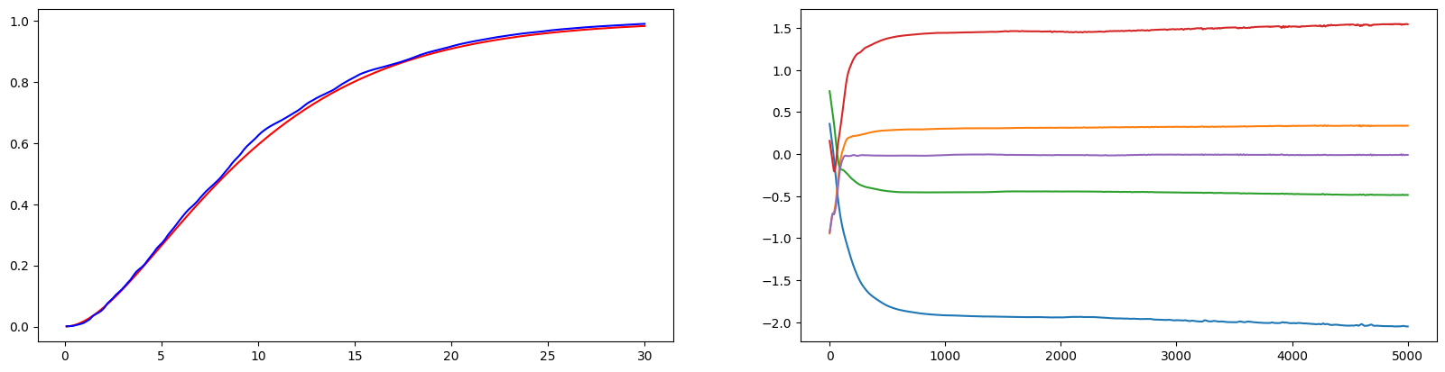
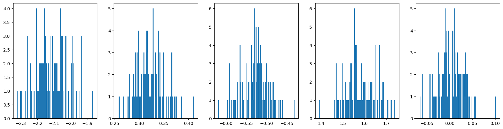
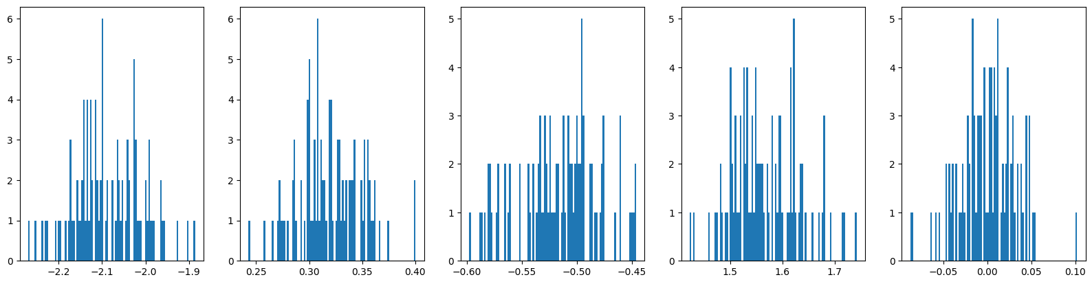
또한 의 각 성분 모두 본래 True 값에 근접하게 학습되었음을 확인할 수 있다.
같은 과정을 에 대해 진행하였다.
# 모델학습 _ L추정 _ replication
y_rate_LC = []
L_errorC = []
L_betaC_x = [[0] for _ in range(common_param['context_size'])]
L_betaC_y = [[] for _ in range(common_param['context_size'])]
L_betaC_res = []
p = np.linspace(0.1, 30, 200)
P = torch.tensor(p, dtype=torch.float).reshape(-1, 1).to(device)
X = torch.zeros((200, common_param['context_size']), dtype=torch.float).to(device)
baseX = torch.zeros((common_param['num_sample'], common_param['context_size']), dtype=torch.float).to(device)
gtC = st.gamma.cdf(p, a=2, loc=0, scale=5).reshape(-1, 1)
for idx in range(1, num_repl+1):
RandomFix(idx)
print(f"====={idx} Replication =====")
breaker = False
modelL = MonoNet_mul(common_param['context_size'])
modelL.to(device)
optimizer = torch.optim.Adam(modelL.parameters(), lr=common_param['learning_rate'])
if idx == 1:
for m in modelL.modules():
if isinstance(m, nn.Linear):
for i in range(common_param['context_size']):
L_betaC_y[i].append(m.weight[0].cpu().detach().numpy()[i])
train_x, train_p, train_y = generate_dataC(common_param['num_sample'])
train_x = train_x.to(device)
train_p = train_p.to(device)
train_y = train_y.reshape(-1, 1).to(device)
for epoch in range(1, common_param['num_epoch']+1):
modelL.train()
L_x, L_0, cox = modelL(train_x, train_p)
L_00 = modelL(baseX, train_p)[0]
loss1 = torch.mean(train_y * L_x - (1-train_y) * torch.log(1 - torch.exp(-L_x)))
loss2 = torch.mean((torch.exp(-L_00 * cox) - torch.exp(-L_x))**2)
train_loss = loss1 + loss2
if torch.any(torch.isnan(train_loss)):
breaker = True
break
if epoch % 100 == 0:
print(f" [Epoch {epoch}] Train loss : {train_loss}")
optimizer.zero_grad()
train_loss.backward()
optimizer.step()
if idx == 1:
for m in modelL.modules():
if isinstance(m, nn.Linear):
cand = m.weight[0].cpu().detach().numpy()
for i in range(common_param['context_size']):
if cand[i] != L_betaC_y[i][-1]:
L_betaC_x[i].append(epoch)
L_betaC_y[i].append(cand[i])
if breaker:
continue
for m in modelL.modules():
if isinstance(m, nn.Linear):
L_betaC_res.append(m.weight[0].cpu().detach().numpy())
F_0 = 1 - torch.exp(-modelL(X, P)[1])
L_errorC.append(gtC - F_0.cpu().detach().numpy())
y_rate_LC.append(sum(train_y.cpu().detach()) / common_param['num_sample'])
fig = plt.figure()
fig.set_figwidth(20)
ax1 = fig.add_subplot(121)
ax1.plot(p, gtC, 'r')
ax1.plot(p, -1 * sum(L_errorC)/len(L_errorC) + gtC, color='b')
ax2 = fig.add_subplot(122)
for i in range(common_param['context_size']):
ax2.plot(L_betaC_x[i], L_betaC_y[i])
fig2 = plt.figure()
fig2.set_figwidth(20)
L_betaC_res = np.array(L_betaC_res).T
for i in range(common_param['context_size']):
globals()[f'ax2{i}'] = fig2.add_subplot(1, common_param['context_size'], i+1)
globals()[f'ax2{i}'].hist(L_betaC_res[i], bins=100)
print(f"y_t=1 비율 : {sum(y_rate_LC).numpy()/len(y_rate_LC)}")
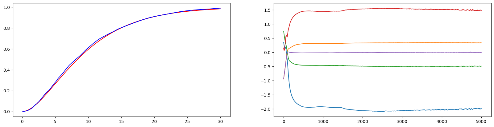
print(f"Std(RMSE) : {np.sqrt(np.mean(sum(val**2 for val in L_errorC)))}")비슷한 학습결과 또한 얻을 수 있었다.
실험3. ic_sp 모델과의 비교
R의 icenReg 패키지의 ic_sp 모델은 지금까지의 실험과 완전히 똑같은 기능을 제공한다. Contextual vector 와 가 주어졌을 때 ic_sp 모델을 통해 와 의 각 변수가 미치는 영향(=가중치 값, )을 알 수 있다.
같은 데이터를 사용하여 두 모델을 학습시키고 결과를 비교하자. 랜덤 시드를 고정하고 데이터를 생성, 저장한다.
# 데이터 생성
import torch
import numpy as np
import pandas as pd
import scipy.stats as st
import matplotlib.pyplot as plt

# Seed 고정 함수
def RandomFix(random_seed):
    torch.manual_seed(random_seed)
    torch.cuda.manual_seed(random_seed)
    np.random.seed(random_seed)
device = torch.device("cuda" if torch.cuda.is_available() else "cpu")
print(device)

class RV_Sampler(st.rv_continuous):
    def __init__(self, cox):
        super().__init__()
        self.cox = cox

    def _cdf(self, x):
        return 1 - (st.gamma.sf(x=x, a=2, loc=0, scale=5))**self.cox

def generate_dataC(num_sample):
    beta = np.array([-2, 0.3, -0.5, 1.5, 0])
    x_t = np.random.randn(len(beta), num_sample)

    cox_t = np.exp(np.dot(beta, x_t))
    v_t = np.array([RV_Sampler(cox=val).rvs(size=1)[0] for val in cox_t])
    p_t = st.uniform.rvs(size=num_sample) * 30
    y_t = (v_t >= p_t).astype(int)

    return x_t.T, p_t.T, y_t.T

# 데이터 -> csv 변환
train_x, train_p, train_y = generate_dataC(10000)
data = np.concatenate([train_x, train_p.reshape(-1, 1), train_y.reshape(-1, 1)], axis=1)

data_pd = pd.DataFrame(data, columns = ['x1', 'x2', 'x3', 'x4', 'x5', 'p', 'y'])
# data_pd.to_csv('data_pd.csv', index=False)
MonoNet를 활용하여 와 를 추정한다.
class MonoBlock(Module):
    def __init__(self, in_feature:int, out_feature:int, mono_indicator = 'inc', activation = 'none', activation_partition = (0,0,1)):
        super().__init__()
        self.activation = activation
        self.activation_partition = activation_partition

        self.in_feature = in_feature
        self.out_feature = out_feature
        self.mono_indicator = mono_indicator

        self.W = Parameter(torch.randn(self.in_feature, self.out_feature))
        self.b = Parameter(torch.randn(self.out_feature))

    def get_activation(self):
        convex = getattr(F, self.activation)
        def concave(x):
            return -convex(-x)
        def saturated(x):
            plus = -convex(-x+torch.ones_like(x)) + convex(torch.ones_like(x))
            minus = convex(x+torch.ones_like(x)) - convex(torch.ones_like(x))
            return torch.where(x >= 0, plus, minus)
        return convex, concave, saturated

    def activation_index(self, x):
        if sum(self.activation_partition) != 1:
            raise ValueError(f"sum of activation_partition must be 1")
        if len(self.activation_partition) != 3:
            raise ValueError(f"length of activation_partition must be 3")

        convex_num = int(self.activation_partition[0] * len(x.T))
        concave_num = int(self.activation_partition[1] * len(x.T))
        return convex_num, convex_num+concave_num, len(x.T)

    def forward(self, x):
        if len(x.shape) == 1:
            x = x.reshape(-1, 1)
        if self.mono_indicator == 'inc':
            self.mono_indicator = torch.ones(x.shape[1])
        if x.shape[1] != self.in_feature:
            raise ValueError(f"matrix multiplication cannot be implemented : {x.shape[0]}x{x.shape[1]} and {self.in_feature}x{self.out_feature}")
        if len(self.mono_indicator) != self.in_feature:
            raise ValueError(f"number of variable does not match : {len(self.mono_indicator)} and {self.in_feature}")

        mono_oper = torch.tensor(self.mono_indicator).to(device).reshape(-1, 1) * torch.abs(self.W)
        W_oper = torch.where(torch.abs(mono_oper) >= torch.abs(self.W), mono_oper, self.W)
        x = torch.matmul(x, W_oper) + self.b

        convex_idx, concave_idx, saturated_idx = self.activation_index(x)
        if self.activation == 'none':
            out = torch.cat([x.T[:convex_idx], x.T[convex_idx:concave_idx], x.T[concave_idx:saturated_idx]], dim=0).T
        else:
            convex_act, concave_act, saturated_act = self.get_activation()
            out = torch.cat([convex_act(x.T[:convex_idx]), concave_act(x.T[convex_idx:concave_idx]), saturated_act(x.T[concave_idx:saturated_idx])], dim=0).T

        return out


class MonoNet_bdd(nn.Module):
    def __init__(self, context_size):
        super().__init__()
        self.context_size = context_size
        self.linear = nn.Linear(self.context_size, 1, bias=False)
        self.mono = nn.Sequential(
            MonoBlock(1+self.context_size, 32, mono_indicator=[*[0]*self.context_size, -1], activation='elu', activation_partition=(0, 0, 1)),
            MonoBlock(32, 16, activation='elu', activation_partition=(0, 0, 1)),
            MonoBlock(16, 8, activation='elu', activation_partition=(0, 0, 1)),
            MonoBlock(8, 1)
        )
        for m in self.modules():
            if isinstance(m, MonoBlock):
                torch.nn.init.uniform_(m.W)
                torch.nn.init.uniform_(m.b, a=-1, b=1)
            elif isinstance(m, nn.Linear):
                torch.nn.init.uniform_(m.weight, a=-1, b=1)

    def coxfunc(self, x):
        return torch.exp(self.linear(x))

    def forward(self, x, p):
        cat = torch.cat([x, p.reshape(-1, 1)], dim=1)
        S_x = torch.sigmoid(self.mono(cat))

        cox = self.coxfunc(x)
        S_0 = S_x**(1/cox)
        return S_x, S_0, cox
# MonoNet에 의한 F_0 추정
comparison = {'learning_rate' : 0.01,
'num_epoch' : 5000,
'num_sample' : 10000,
'context_size' : 5}
RandomFix(1)
baseX = torch.zeros((comparison['num_sample'], comparison['context_size']), dtype=torch.float).to(device)
modelS = MonoNet_bdd(comparison['context_size'])
modelS.to(device)
optimizer = torch.optim.Adam(modelS.parameters(), lr=comparison['learning_rate'])
train_x = torch.tensor(train_x, dtype=torch.float).to(device)
train_p = torch.tensor(train_p.reshape(-1, 1), dtype=torch.float).to(device)
train_y = torch.tensor(train_y.reshape(-1, 1), dtype=torch.float).to(device)
for epoch in range(1, comparison['num_epoch']+1):
modelS.train()
S_x, S_0, cox = modelS(train_x, train_p)
S_00 = modelS(baseX, train_p)[0]
loss1 = torch.mean(-1 * train_y * torch.log(S_x) - (1-train_y) * torch.log(1 - S_x))
loss2 = torch.mean((S_00**cox - S_x)**2)
train_loss = loss1 + loss2
if epoch % 100 == 0:
print(f" [Epoch {epoch}] Train loss : {train_loss}")
optimizer.zero_grad()
train_loss.backward()
optimizer.step()
for m in modelS.modules():
if isinstance(m, nn.Linear):
print(m.weight[0].cpu().detach().numpy())
p = np.linspace(0.1, 30, 200)
P = torch.tensor(p, dtype=torch.float).reshape(-1, 1).to(device)
X = torch.zeros((200, comparison['context_size']), dtype=torch.float).to(device)
gtC = st.gamma.cdf(p, a=2, loc=0, scale=5).reshape(-1, 1)
S_0 = modelS(X, P)[0].cpu().detach().numpy()
plt.plot(p, gtC, color='r')
plt.plot(p, S_0, color='b')추정한 결과는 다음과 같다.
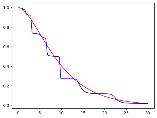
- 추정한
같은 데이터를 icenReg 패키지의 ic_sp 모델에 학습시키자. 다음은 R 코드로 작성되었다.
install.packages('icenReg')
library('icenReg')
library("utils")

data_pd <- read.csv('/content/data_pd.csv')
data_pd$p <- as.numeric(as.character(data_pd$p))
data_pd$y <- 3 * (1 - data_pd$y )
data_pd$q <- data_pd$p

data_pd$q[data_pd$y == 0] <- Inf
data_pd$p[data_pd$y == 3] <- 0

data_pd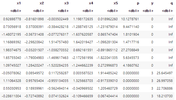
- data_pd의 일부이다.
- type-I interval censored data임을 표시하기 위해 y열을 수정하고, q열을 만들어 [p, q]의 interval을 구성하였다.
fit_ph <- ic_sp(formula = Surv(time=p, time2=q, event=y, type='interval') ~ x1+x2+x3+x4+x5, model = 'ph', bs_samples = 100, data = data_pd)

newdata <- data.frame(x1 = c(0),
                      x2 = c(0),
                      x3 = c(0),
                      x4 = c(0),
                      x5 = c(0))
alpha = 2
theta = 5

plot(data.frame(x = 0:300 / 10, prob = 1 - pgamma(q = 0:300 / 10, shape = alpha, scale = theta, lower.tail = TRUE)), lwd=2, type="l", col='red')
par(new=TRUE)
plot(fit_ph, newdata, lwd=2, col='blue')- 모델을 학습시키고 을 대입한 그래프를 표현하였다.
- 시각적 용이함을 위해 두 그래프를 겹쳐 표현하였다.
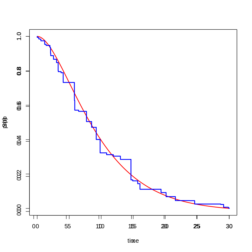
- 붉은 색은 True , 푸른 색은 추정한 이다.
- 추정한
두 모델의 결과는 비슷하지만, 육안으로 보았을 때 ic_sp 모델이 를 더욱 잘 추정했다고 말할 수 있겠다. 이는 Neural Network를 더 깊게 구성함으로써 충분히 보완할 수 있을 것이다.
5. Conclusion
지금까지 Contextual Pricing을 위한 Neural Network 모델을 설계하고 실험을 진행하였다. 마지막 실험을 마친 후, ic_sp라는 좋은 모델이 이미 있는데, 굳이 Neural Network로 구현할 의미가 있을까? 라는 생각이 들 수 있을 것이다.
하지만 Neural Network의 높은 자유도에 그 의의가 있다고 생각한다. 가령 Loss Fuction에 를 더함으로써 추정치의 대략적인 범위를 조정하는 등의 추가적인 액션이 가능하다는 것이다.
현재 Neural Network에서 생각해봐야할 점은 identifiability이다. 하나의 함수를 추정하는 일반적인 Neural Network 문제와 달리, 지금은 두 개의 함수()를 각각 정확히 추정해야 한다. 그렇기에 를 추정하도록 하는 만으로는 두 함수를 구분해낼 수 없고, 그 역할을 를 통해 이루어냈다. 이러한 의 구성이 이론적으로 identifiability을 보장할 수 있는가가 추가적으로 논의되어야 할 점이다.