[통계] 회귀(Regression)

📁 단순선형회귀

✔️ 한개의 변수에 의한 결과를 예측

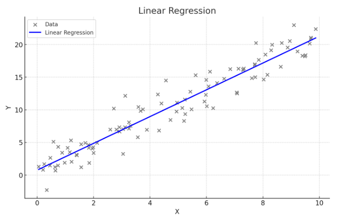
• 하나의 독립 변수(X)와 하나의 종속 변수(Y) 간의 관계를 직선으로 모델링하는 방법
  

<회귀식>

• Y = β0 + β1X, 여기서 β0는 절편, β1는 기울기
• 중학교 때 배웠던 1차함수와 비슷

<특징>

• 독립 변수의 변화에 따라 종속 변수가 어떻게 변화하는지 설명하고 예측
• 데이터가 직선적 경향을 따를 때 사용
• 간단하고 해석이 용이
• 데이터가 선형적이지 않을 경우 적합하지 않음

<단순선형회귀는 어떨 때 사용할까?>

• 하나의 독립변수와 종속변수와의 관계를 분석 및 예측
  • 광고비(X)와 매출(Y) 간의 관계 분석
  • 현재의 광고비를 바탕으로 예상되는 매출을 예측 가능

import numpy as np
import pandas as pd
import matplotlib.pyplot as plt
from sklearn.linear_model import LinearRegression
from sklearn.model_selection import train_test_split
from sklearn.metrics import mean_squared_error, r2_score

# 예시 데이터 생성
np.random.seed(0)
X = 2 * np.random.rand(100, 1)
y = 4 + 3 * X + np.random.randn(100, 1)

# 데이터 분할
X_train, X_test, y_train, y_test = train_test_split(X, y, test_size=0.2, random_state=42)

# 단순선형회귀 모델 생성 및 훈련
model = LinearRegression()
model.fit(X_train, y_train)

# 예측
y_pred = model.predict(X_test)

# 회귀 계수 및 절편 출력
print("회귀 계수:", model.coef_)
print("절편:", model.intercept_)

# 모델 평가
mse = mean_squared_error(y_test, y_pred)
r2 = r2_score(y_test, y_pred)
print("평균 제곱 오차(MSE):", mse)
print("결정 계수(R2):", r2)

# 시각화
plt.scatter(X, y, color='blue')
plt.plot(X_test, y_pred, color='red', linewidth=2)
plt.title('linear regeression')
plt.xlabel('X : cost')
plt.ylabel('Y : sales')
plt.show()

---

📁 다중선형회귀

✔️ 두 개 이상의 변수에 의한 결과를 예측

<다중선형회귀란 무엇인가?>

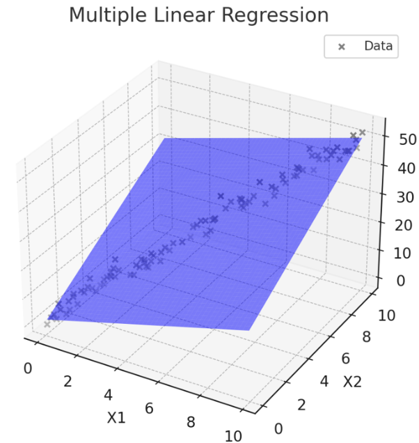
• 두 개 이상의 독립 변수(X1, X2, ..., Xn)와 하나의 종속 변수(Y) 간의 관계를 모델링
  

<회귀식>

• Y = β0 + β1X1 + β2X2 + ... + βnXn

<특징>

• 여러 독립 변수의 변화를 고려하여 종속 변수를 설명하고 예측
• 종속변수에 영향을 미치는 여러 독립변수가 있을 때 사용
• 여러 변수의 영향을 동시에 분석할 수 있음
• 변수들 간의 다중공선성 문제가 발생할 수 있음

💡 다중공선성

• 회귀분석에서 독립 변수들 간에 높은 상관관계가 있는 경우
• 이는 회귀분석 모델의 성능과 해석에 여러 가지 문제를 일으킬 수 있음
  • 독립 변수들이 서로 강하게 상관되어 있으면, 각 변수의 개별적인 효과를 분리해내기 어려워져 회귀의 해석을 어렵게 만듬
  • 다중공선성으로 인해 실제로 중요한 변수가 통계적으로 유의하지 않게 나타날 수 있음
• 어떻게 진단할 수 있을까?
  • 가장 간단한 방법으로는 상관계수를 계산하여 상관계수가 높은(약 0.7) 변수들이 있는지 확인해볼 수 있음
  • 더 정확한 방법으로는 분산 팽창 계수 (VIF)를 계산하여 VIF값이 10이 높은지 확인하는 방법으로 다중공선성이 높다고 판단할 수 있음
• 다중공선성 해결 방법
  • 가장 간단한 방법으로는 높은 계수를 가진 변수 중 하나를 제거하는 것
  • 혹은 주성분 분석(PCA)과 같은 변수들을 효과적으로 줄이는 차원 분석 방법을 적용하여 해결할 수도 있음

<다중선형회귀는 어떨 때 사용할까?>

• 두 개 이상의 독립 변수와 종속변수와의 관계를 분석 및 예측
  • 다양한 광고비(TV, Radio, Newspaper)과 매출 간의 관계 분석
  • 현재의 광고비(TV, Radio, Newspaper)를 바탕으로 예상되는 매출을 예측 가능

# 예시 데이터 생성
data = {'TV': np.random.rand(100) * 100,
        'Radio': np.random.rand(100) * 50,
        'Newspaper': np.random.rand(100) * 30,
        'Sales': np.random.rand(100) * 100}
df = pd.DataFrame(data)

# 독립 변수(X)와 종속 변수(Y) 설정
X = df[['TV', 'Radio', 'Newspaper']]
y = df['Sales']

# 데이터 분할
X_train, X_test, y_train, y_test = train_test_split(X, y, test_size=0.2, random_state=42)

# 다중선형회귀 모델 생성 및 훈련
model = LinearRegression()
model.fit(X_train, y_train)

# 예측
y_pred = model.predict(X_test)

# 회귀 계수 및 절편 출력
print("회귀 계수:", model.coef_)
print("절편:", model.intercept_)

# 모델 평가
mse = mean_squared_error(y_test, y_pred)
r2 = r2_score(y_test, y_pred)
print("평균 제곱 오차(MSE):", mse)
print("결정 계수(R2):", r2)

---

📁 범주형 변수

✔️ 회귀에서 범주형 변수의 경우 특별히 변환을 해주어야 함!

<회귀에서의 범주형 변수>

• 범주형 변수
  • 수치형 데이터가 아닌 주로 문자형 데이터로 이루어져 있는 변수가 범주형 변수
• 범주형 변수 종류
• ex) 성별(남, 여), 지역(도시, 시골) 등이 있으며, 더미 변수로 변환하여 회귀 분석에 사용
  • 순서가 있는 범주형 변수
    • 옷의 사이즈 (L, M, …), 수능 등급 (1등급, 2등급, ….)과 같이 범주형 변수라도 순서가 있는 변수에 해당
    • 이런 경우 각 문자를 임의의 숫자로 변환해도 문제가 없음 (순서가 잘 반영될 수 있게 숫자로 변환)
    • ex) XL → 3, L → 2, M → 1, S → 0
  • 순서가 없는 범주형 변수
    • 성별 (남,여), 지역 (부산, 대구, 대전, …) 과 같이 순서가 없는 변수에 해당
    • 2개 밖에 없는 경우 임의의 숫자로 바로 변환해도 문제가 없지만
    • 3개 이상인 경우에는 무조건 원-핫 인코딩(하나만 1이고 나머지는 0인 벡터)변환을 해주어야 함 → pandas의 get_dummies를 활용하여 쉽게 구현 가능
    • ex) 부산 = [1,0,0,0], 대전 = [0,1,0,0], 대구 = [0,0,1,0], 광주 = [0,0,0,1]

<범주형 변수는 어떻게 사용할까?>

• 범주형 변수를 찾고 더미 변수로 변환한 후 회귀 분석 수행
  • 성별, 근무 경력과 연봉 간의 관계
  • 성별과 근무 경력이라는 요인변수 중 성별이 범주형 요인변수에 해당
  • 해당 변수를 더미 변수로 변환
  • 회귀 수행

# 예시 데이터 생성
data = {'Gender': ['Male', 'Female', 'Female', 'Male', 'Male'],
        'Experience': [5, 7, 10, 3, 8],
        'Salary': [50, 60, 65, 40, 55]}
df = pd.DataFrame(data)

# 범주형 변수 더미 변수로 변환
df = pd.get_dummies(df, drop_first=True)

# 독립 변수(X)와 종속 변수(Y) 설정
X = df[['Experience', 'Gender_Male']]
y = df['Salary']

# 단순선형회귀 모델 생성 및 훈련
model = LinearRegression()
model.fit(X, y)

# 예측
y_pred = model.predict(X)

# 회귀 계수 및 절편 출력
print("회귀 계수:", model.coef_)
print("절편:", model.intercept_)

# 모델 평가
mse = mean_squared_error(y, y_pred)
r2 = r2_score(y, y_pred)
print("평균 제곱 오차(MSE):", mse)
print("결정 계수(R2):", r2)

---

📁 다항회귀, 스플라인 회귀

✔️ 데이터가 훨씬 복잡할 때 사용하는 회귀!

<다항회귀, 스플라인 회귀란 무엇인가?>

• 다항회귀

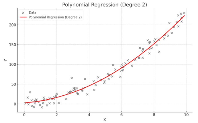
  • 독립 변수와 종속 변수 간의 관계가 선형이 아닐 때 사용. 독립 변수의 다항식을 사용하여 종속 변수를 예측
  • 데이터가 곡선적 경향을 따를 때 사용
  • 비선형 관계를 모델링할 수 있음
  • 고차 다항식의 경우 과적합(overfitting) 위험이 있음
    

• 스플라인 회귀

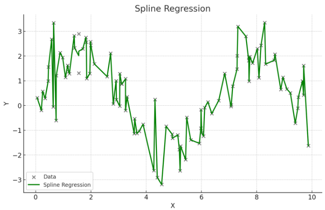
  • 독립 변수의 구간별로 다른 회귀식을 적용하여 복잡한 관계를 모델링
  • 구간마다 다른 다항식을 사용하여 전체적으로 매끄러운 곡선을 생성
  • 데이터가 국부적으로 다른 패턴을 보일 때 사용
  • 복잡한 비선형 관계를 유연하게 모델링할 수 있음
  • 적절한 매듭점(knots)의 선택이 중요

<다항회귀는 어떨 때 사용할까?>

• 독립변수와 종속변수의 관계가 비선형 관계일 때 사용
  • 주택 가격 예측(면적과 가격 간의 비선형 관계)

from sklearn.preprocessing import PolynomialFeatures

# 예시 데이터 생성
np.random.seed(0)
X = 2 - 3 * np.random.normal(0, 1, 100)
y = X - 2 * (X ** 2) + np.random.normal(-3, 3, 100)
X = X[:, np.newaxis]

# 다항 회귀 (2차)
polynomial_features = PolynomialFeatures(degree=2)
X_poly = polynomial_features.fit_transform(X)

model = LinearRegression()
model.fit(X_poly, y)
y_poly_pred = model.predict(X_poly)

# 모델 평가
mse = mean_squared_error(y, y_poly_pred)
r2 = r2_score(y, y_poly_pred)
print("평균 제곱 오차(MSE):", mse)
print("결정 계수(R2):", r2)

# 시각화
plt.scatter(X, y, s=10)
# 정렬된 X 값에 따른 y 값 예측
sorted_zip = sorted(zip(X, y_poly_pred))
X, y_poly_pred = zip(*sorted_zip)
plt.plot(X, y_poly_pred, color='m')
plt.title('polynomial regerssion')
plt.xlabel('area')
plt.ylabel('price')
plt.show()