[ICLR 2020] N-BEATS : Neural Basis Expansion Analysis for Interpretable Time Sereis Forecasting

진서연 ·2023년 3월 14일

N-BEATS Time Series iclr2020 paper reading

Paper Reading

목록 보기

4/24

Abstract

이 논문의 목적은 solving the univariate time series point forecasting problem using deep learning이다. 단변량 시계열 예측은 많은 연구가 되어왔는데, 이 논문에서 이를 강조하는 이유는 기존의 통계 기반의 모델과 달리 순수 deep learning을 이용한 모델이기 때문이다.

이 외에도 이 모델은 아래의 장점들을 가지고 있다.

being interpretable (특히 이 부분에 집중해서 볼필요가 있다.)
applicable without modification to a wide array of target domains
fast to train

Introduction

NLP, CV처럼 현재 산업에 entrenched 된 분야와는 달리 TS forecasting이 통계 기반의 모델을 이기기위한 노력들이 있다. M4 대회 우승 모델은 neural residual/attention dilated LSTM 와 classical Holt-Winters statistical model이 결합된 형태이고, Holt-Winters component가 있어서 더 정확해진다는 분석이 가능해진다.

→ 이 논문에서는 pure DL로 시계열 데이터예측에 대한 interpretable한 feature extract와 정확한 예측을 목표로 함.

이 논문에서 계속 이야기하는 M3,M4 competition 링크

https://forecasters.org/resources/time-series-data/

Problem Statement

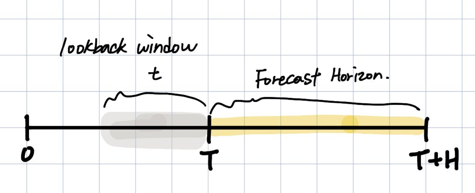
우리는 lookback window길이만큼의 과거 데이터를 통해서 forecast horizon H 길이를 예측함.

아래와 같은 metric으로 performance를 평가한다.

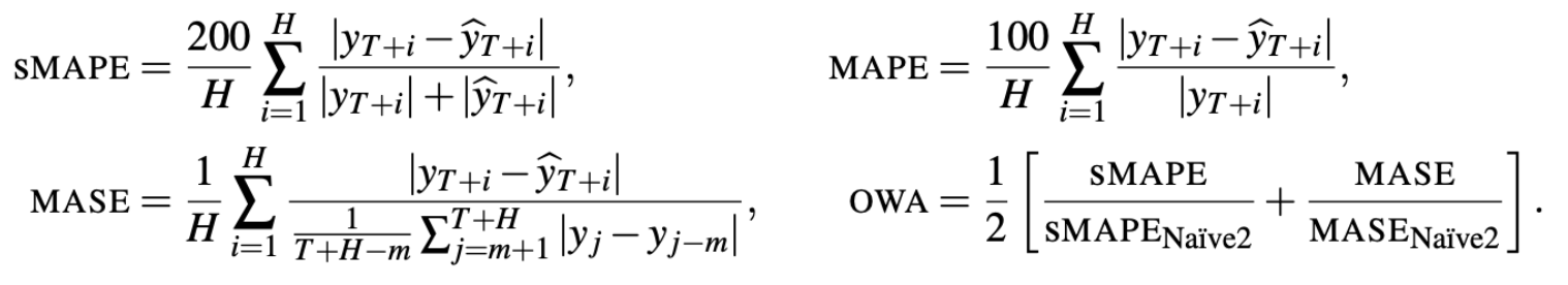
sMAPE와 MASE는 scale-free metric이다. sMAPE같은 경우 predicted value와 ground truth사이의 평균으로 error를 scaling한다.

MASE에서의 m은 data의 periodicity이다. 예를 들어 월 데이터는 12의 주기성을 갖는다.

OWA는 M4 competition에서 사용되는 metric이다.

N-BEATS

Basic block

모델은 간단하고 일반적이어야하며, 깊어야한다(expressive and deep)
feature engineering or input scaling에 영향받지 않아야한다.
해석가능한 출력 값이 나오도록 해야한다. (사람들이 직관적으로 알아볼 수 있도록)

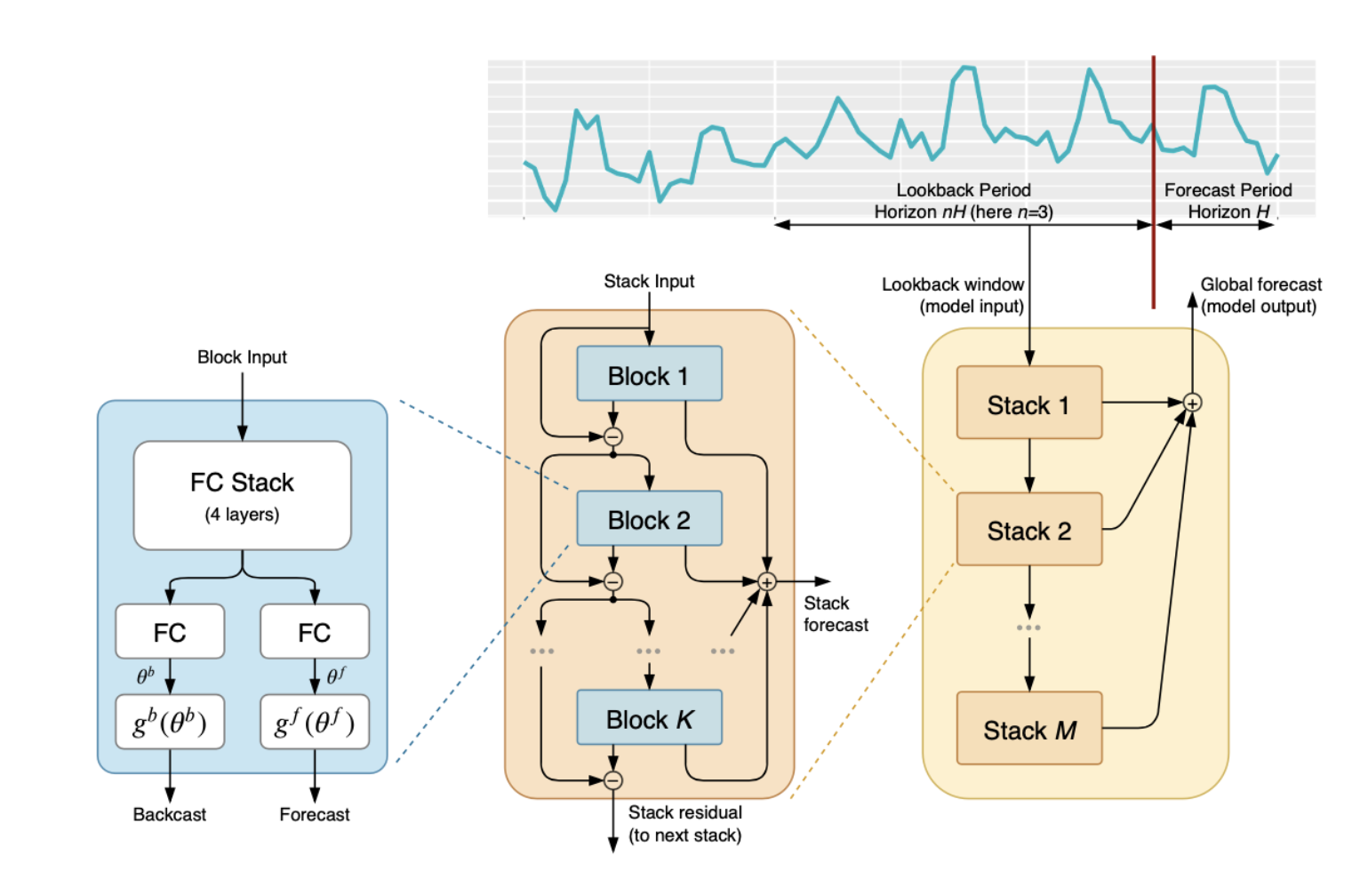
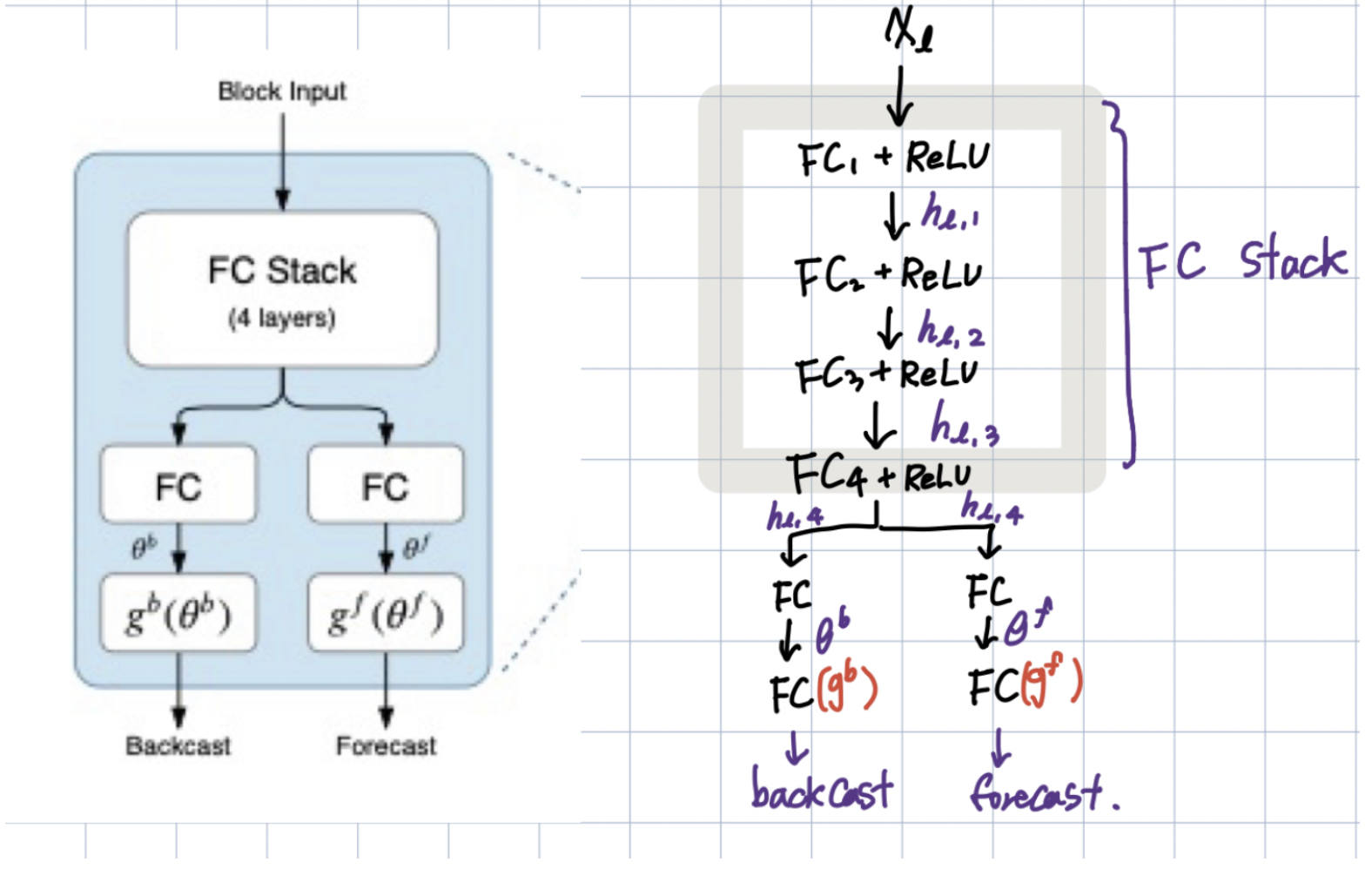
논문에서는 가장 왼쪽의 block 구조를 l번째 block이라고 가정한다.

입력으로는 lookback period의 데이터를 전부 받고, 출력으로는 backcast와 forecast를 한다.

이해를 위해 만약 20일의 데이터를 보고 다음 10을 예측한다면, 여기서 lookback period는 20이고, forecast Period는 10이 된다.

이야기하고 있는 파란색의 block은 두가지 파트로 나누어져있는데,

forward와 backward를 만드는 FC(Fully-Connected layer)와
backcast, forecast를 생성하기 위해서 내부적으로 투영한다.

Backcast 벡터의 의미는 해당 Block에서 생성한 회귀관측값(20개)을 의미한다.

Forecast 벡터의 의미는 예측한 10개의 값을 의미한다.

논문에서는 파란색 basic block에 대해서 아래와 같이 보여준다.

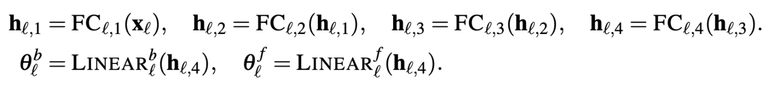
이 표기들을 토대로 그린 네트워크 구조!. (참고)

첫번째 파트 :

basic block은 궁극적으로는 $\theta^f_l$ 을 예측하는 것, (궁극적인 목표는 $g^f_l$ 와의 적절한 mixing으로 $\hat{y}$ 을 정확하게 예측하는 것!)

$\theta^g_l$ 을 이용한 sub-network을 이용하여 예측에 필요하지 않은 input의 성분을 제거하여 downstream block을 돕는다.

두번째 파트 :

function g에 부분으로 $\theta^f_l , \theta^g_l$ 을 basis layer를 통해서 output으로 만든다.

output은 아래의 수식들로 나타내었는데, 여기서 $v^f_i, v^g_i$ 는 basis vector를 나타낸다.

Doubly Residual Stacking

1. tranditional residual network : 층의 입력과 출력을 더해서 다음 층으로 넘겨줌. 

2. DenseNet : 모든 stack과의 추가적인 연결을 통해서 tranditional residual network 원리 확장시킴. 

→ DenseNet은 trainability 향상하지만, **해석하기 어려운 모델이라는 단점이 있다. (이 논문에서는 해석가능성에 대해서 강조를 하기 때문에 이러한 점에서 DenseNet을 향상시키는 것이 큰 contribution이라고 생각했을 것.)**

해석가능하게 하기 위해서 doubly residual stacking 모델을 제안한다.

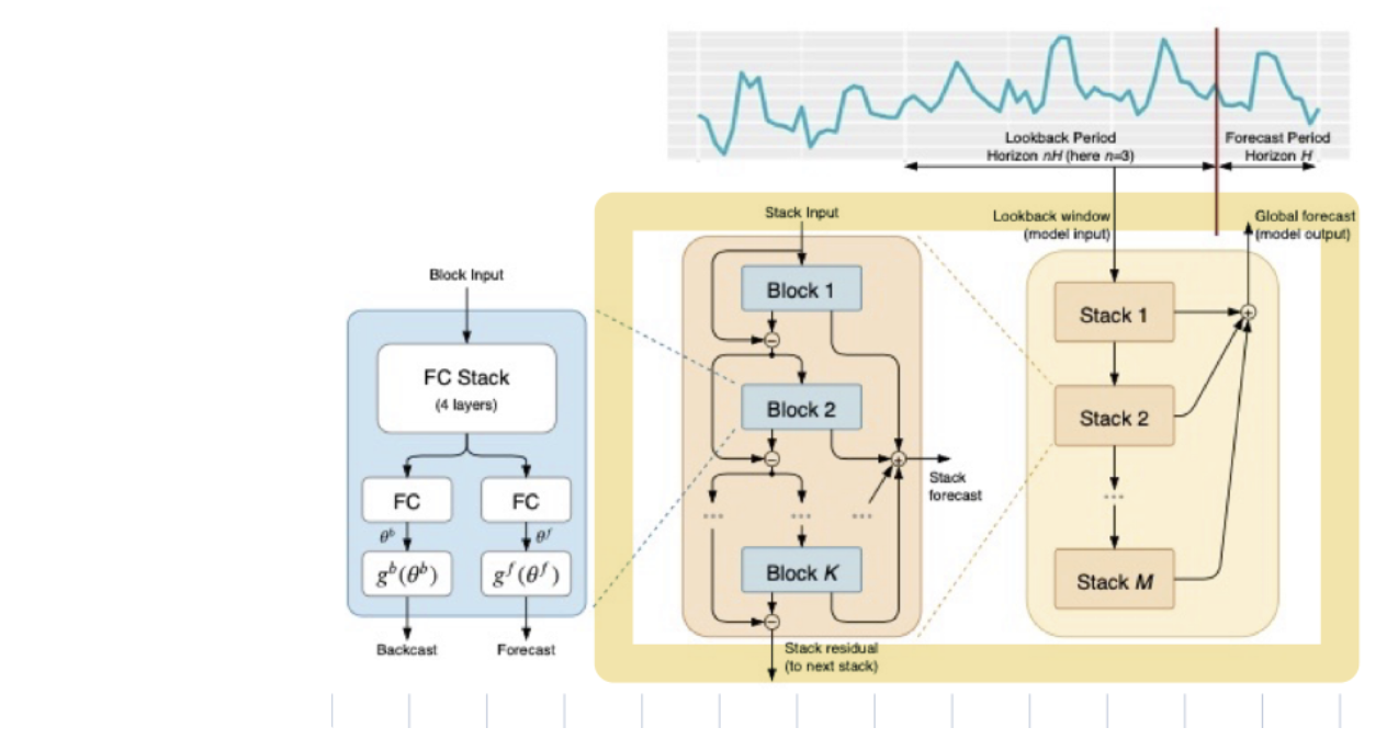
위의 그림에서는 노란색 박스로 그려놓은 부분들에 해당한다.

“doubly”라는 모델이름에서도 알 수 있듯, 이 논문에서 제안한 모델은 두가지 residual branch로 이루어져있다.

backcast prediction
forecast branch로 이루어져있다.

이 부분에서의 key point

forcast,backcast에 적용된 doubly Residual connection 구조는 gradient backpropagation이 더 잘 흐르도록 해줌.
1. Block 1 의 input $x_1$ 은 $x$ 그 자체임.
2. Block 2 ~T 의 input은 input signal의 연속적인 분석으로 생성된 것. (즉, residual branch들을 통과하는 값)
backcast : $x_l = x_{l-1} - \hat{x}_{l-1}$ forecast : $\hat{y} =\sum_l \hat{y}_l$
1. backcast 에서 $\hat{x}_{l-1}$ (이전 Block의 예측값)을 빼줌으로써 더 잘 예측하고, downstream block이 더 잘 예측하도록 한다.
2. forecast 에서 $\hat{y}_l$ 은 각 layer에서의 예측값이고 final forecast 값인 $\hat{y}$ 은 전체 값의 summation인데 이러한 구조가 Input을 계층적으로 분해함. → 이런 부분들이 이 모델의 해석력 (Interpretability)를 부여한다.

Interpretability

해석하지 않는 부분
1. $\hat{y}_l = \bold{V^f_l}\theta^f_l + b^f_l$ $\hat{x}_l = \bold{V^b_l}\theta^b_l + b^b_l$ 이 식을 앞에서 설명한 $g^f_l,g^b_l$ 함수이다.
  
  → 위의 수식은 $\bold{v}^f_l,b^f_l$ 을 학습하는것으로 볼 수 있다.
  
  → 여기서 $\bold{v}^f_l$ 의 dimension : $H \times dim(\theta^f_l)$ 인데, first dimension : time index in the forecast domain으로 해석되고, second dimension은 basis function의 index로 해석된다.
  
  : 그래서 $\bold{v}^f_l$ 벡터의 column은 시간영역에서의 waveform으로 볼 수 있고, 이러한 wave form을 학습하기 때문에 해석되지 않는다.
해석하는 부분

해석이 가능한 모델 구조는 앞에서 이야기한 모델의 구성요소를 모두 포함하고 있음.

우리는 Stack output을 쉽게 해석하기위해 모델에 Trend 및 Seasonality decomposition을 설계함.

Trend model

"trend”는 단조증가(또는 감소)하는 현상을 보인다. N-BEATS논문에서는 stack output의 trend 해석이 가능하도록 함
1. Basic block의 $g^b,g^f$ 를 변형해줌으로써, Trend Block을 만듬.
  1. trend mimic을 위해 $g^b,g^f$ 를 작은 차수의 $p$ 의 다항식으로 제한함.
  2. $\hat{y}_{s,l} = \sum^p_{i=0}\theta^f_{s,l,i}t^i$ 이렇게 정의함. ( $p$ 의 다항식)
    1. 여기서 $t = [0,1,2,...,H-2,H-1]^T/H$
  3. 최종적으로 정리하면, $\hat{y}^{tr}_{s,l} = \bold{T}\theta^f_{s,l}$ 로 정의할 수 있다. ( $\bold{T} = [1,t,...,t^p]$ .)
    1. $p$ 가 2,3 처럼 작다면, trend 예측값이 trend를 모방하도록 함.
Seasonality model

"seasonality”란 일정하게 반복되는 주기를 이야기한다. (sin 함수와같은 것들)
1. Basic block의 $g^b,g^f$ 를 변형해줌으로써 Seasonality Block을 만듬.
  1. seasonality를 위해 $g^b,g^f$ 를 periodic function으로 정의함. ( $ex . y_t=y_{t-\Delta}$ )
  2. $\hat{y}_{s,l} = \sum^{\lfloor(H/2) -1\rfloor}_{i=0} \theta^f_{s,l,i}cos(2\pi it)+\theta^f_{s,l,i + \lfloor H/2\rfloor}sin(2\pi it)$
    1. 여기서 사용된 periodic functioin은 Fourier series임.
  3. 최종적으로 정리하면, $\hat{y}^{seas}_{s,l} = \bold{S}\theta^f_{s,l}$ 으로 정리할 수 있다.( $\bold{S} = [1,cos(2\pi t),...,cos(2\pi\lfloor H/2-1\rfloor \bold{t}),sin(2\pi \bold{t}),...,sin(2\pi \lfloor H/2-1\rfloor \bold{t})]$ )
    1. matrix of sinusoidal waveforms.
Summary
1. interpretable architecture : Trend stack → Seasonality stack
2. Doubly residual stack 구조 : Trend stack을 거친 output이 Seasonality Stack에 들어가기전에 Trend component를 제거한다!
3. Trend, Seasonality가 별도로 해석이 가능하다.
4. 각각의 Stack은 block들이 residual connection으로 연결되어있다. 이 논문에서는 이 가각의 block들이 sharing $g^b_{s,l},g^f_{s,l}$ 와 weights를 block들에 걸쳐서 공유하는 것이 더 좋은 성능을 보여준다고 한다.

Ensembling

L2-norm이나 dropout 기법보다 좋은 regularization 기법임.
ensemble 모델은 3가지의 다른 metric(sMAPE,MASE,MAPE)사용.
모든 horizon H마다 각 모델들은 2H ~7H까지 6가지의 다른 window 길이로 학습함.
총합한 ensemble은 multi-scale aspect을 갖게 된다. 이 논문에서는 총 180 종류의 모델을 사용하였고, ensemble을 위하여 median을 사용함.
1. 각 모델들을 전부 다른 random 초기화를 사용하는 baggin 기법을 사용함.

Statistical modeling approaches :
1. advanced variations of exponential smoothing
2. ARIMA,auto-ARIMA
ML/TS combination approaches :
1. statistical engines을 feature로 사용함.
2. variations of RNNs
  1. combinations of RNNs with dilation,residual connections and attention.
  2. Holt-Winters style seasonality model with its parameters fitted to a given TS via gradient descent and a unique combination of dilation/residual/attention approaches for each forecast horizon.

Experimental Results

Experiments Summary

Dataset : M4,M3,Tourism
Baselines : Pure ML,Statistical,ProLogistica,ML/TS combination, DL/TS hybrid
Metric : M4(OWA,sMAPE),M3(sMAPE),Tourism(MAPE)

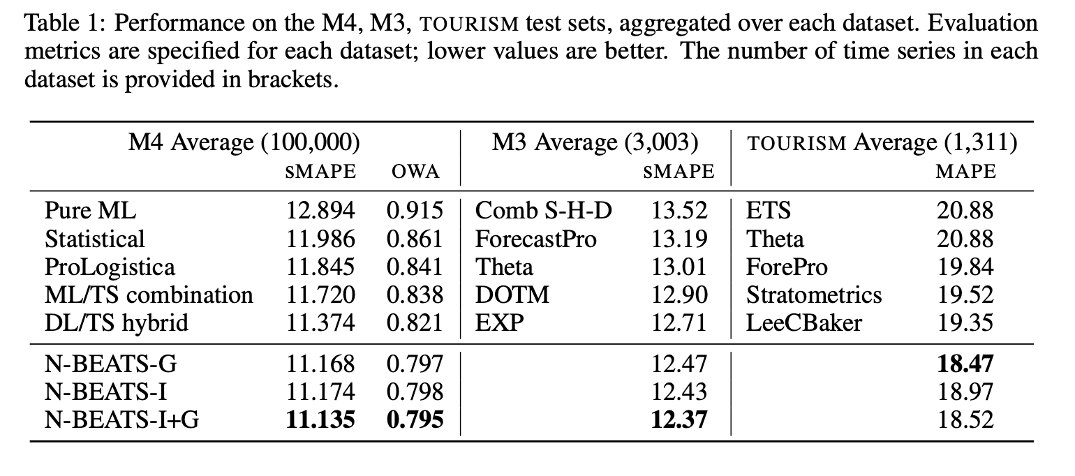
M4 DATASET BASELINES

Pure ML : M4 Competition에 제출된 pure ML 모델들 중에서 가장 좋은 성능의 모델 -
Statistical : best Pure Statistical model -
ML/TS combination : second best entry, gradiente boosted tree + few statistical time series model -
ProLogistica : third entry, weighted ensemble of statistical methods.-
DL/TS hybrid : winner of M4 competition

M3 DATASET BASELINES

Theta : winner of M3 competition
DOTM : Dynamically Optimized Theta Model
EXP : 최신 통계학적 접근방식의 모델
ForecastPro : model selection between exponential smoothing and ARIMA and moving average

Tourism DATASET BASELINES

ETS : Exponential Smoothing with cross-validated additive/multiplicative model
Stratometrics : an unknown technique
LeeCBaker : a weighted combination of Naive, linear trend model, and exponentially weighted least sqaures regression trend.

Dataset

M4 Dataset : The M4 dataset was created by selecting a random sample of 100,000 time series from the ForeDeCk database.
- ForeDeCk database : ForeDeCk is a time series database compiled at the National Technical University of Athens that contains 900,000 continuous time series, built from multiple, diverse and publicly accessible sources. ForeDeCk emphasizes business forecasting applications, including series from relevant domains such as industries, services, tourism, imports & exports, demographics, education, labor & wage, government, households, bonds, stocks, insurances, loans, real estate, transportation, and natural resources & environment.
M3 Dataset : M4 dataset과 유사하지만 더 작다.
Tourism Dataset : Tourism Australia, HongKong Touism board and Tourism New Zealand의 데이터이다.

Training Methodology

would like to stress that models for different horizons and datasets reuse the same architecture. → 대부분의 데이터셋과 다른 horizon에 대해서 동일한 아키텍쳐와 파라미터들로 사용함.

Interpretability results

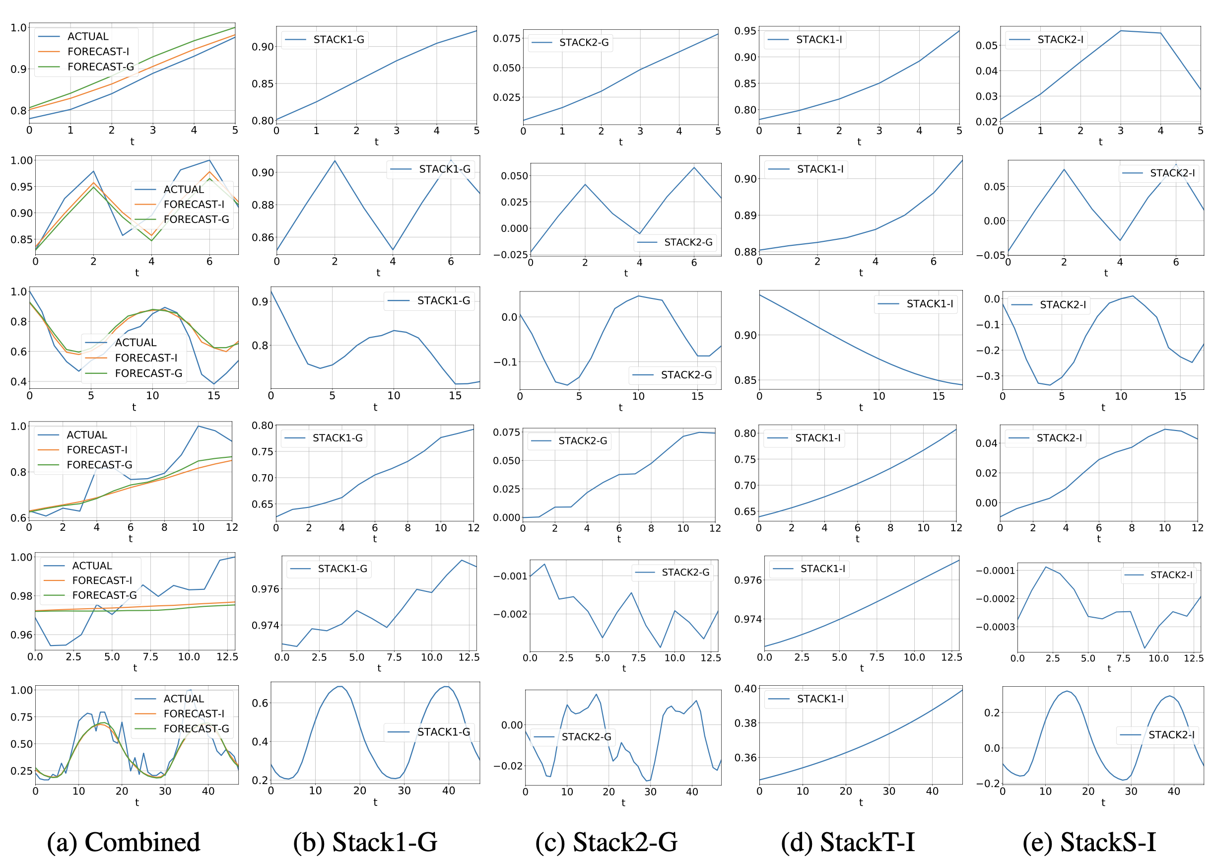
M4 Dataset의 실험 결과

(a)는 실제 actural (ground truth)와 Interpretability model(FORECAST-I) 와 Generic model(FORECAST-G)를 visualization한 것.

(b),(c) → Generic model (해석불가능한 모델) : Stack 1,2의 결과 → FORECAST -G 는 이 두 결과의 합.

(d),(e) → Interpretability model (해석가능한 모델) : FORECAST-I도 이 두 결과의 합.

(d) : Trend 의 경우 monotonic하고, slowly moving하는것들이 보인다.

(e) : Seasonality 의 경우 regular, cyclical하고 역시나 반복되는 주기들을 볼 수 있다.

each row, top to bottom : yearly, quarterly,monthly,weekly,daily,hourly

진서연

SheoYon.Jhin

이전 포스트

[Arxiv 2023] Mitigating Cold-start Problem using Cold Causal Demand Forecasting Model

다음 포스트

[ICLR 2020] N-BEATS : Neural Basis Expansion Analysis for Interpretable Time Sereis Forecasting

Paper Reading

Abstract

Introduction

Problem Statement