CS231n

강의 링크

Data-driven approach

1. collecet a dataset of images and labels
2. use machine learning to train an image classifier
3. evaluate the classifier on a withheld sest of test images
   -> test & evaluate

Nearest Neighbor Classifier

• 모든 training image와 label을 기억하고, input과 가장 비슷한 것의 class를 return하는 classifier

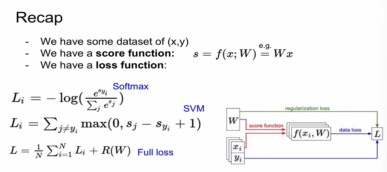
Linear Classification

ex) image captioning = CNN + RNN
CNN - object classification from image
RNN - caption generation (RNN은 sequence 처리에 강한 network임)

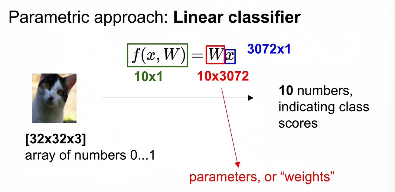
Parametric approach

Linear Classifier가 구분하기 어려운 dataset?

• negative image, grey-scaled image, texture와 shape은 다르지만 색이 같은 경우

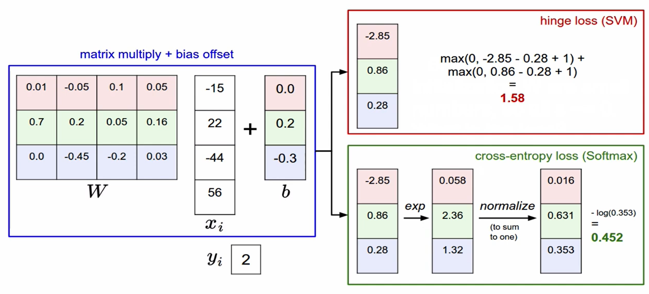
• Linear score function을 정의한 것임. -> loss funcion이 score를 loss로 정량화함.

Loss Function

SVM - Hinge Loss
Softmax - Cross Entropy Loss

Multiclass SVM loss

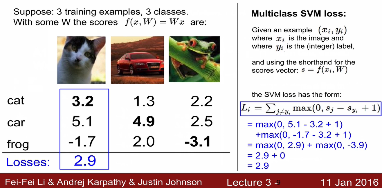
sj: 잘못된 label의 score
syi: 정답 label의 score

• correct label의 score가 incorrect label의 score보다 1 이상 크면 loss = 0
  

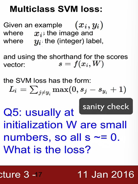
• Sanity check: 초기 loss 값 == (클래스 수) -1
  학습 진행 전 초기 값 확인.

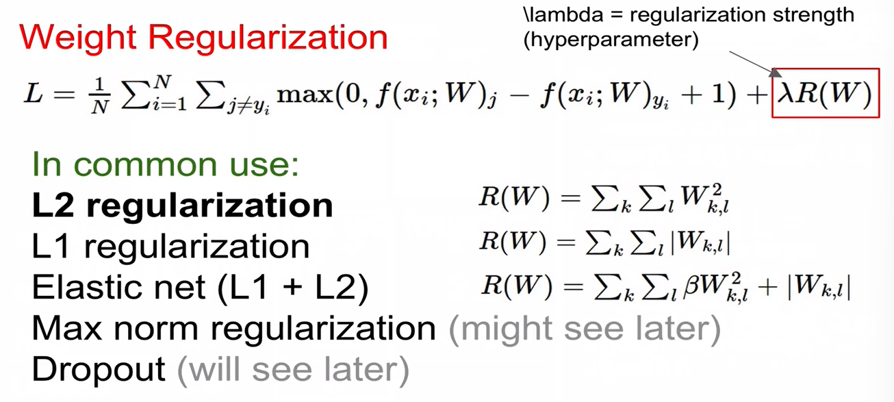
• loss를 0으로 만드는 W의 값이 unique 하지 않다는 버그가 있음. 이를 해결하지 위해 Regularization을 함.

• Regularization 도입 시 training error는 커지겠지만(training data에 대한 performance는 안 좋아지겠지만) test set performance는 더 좋아짐.

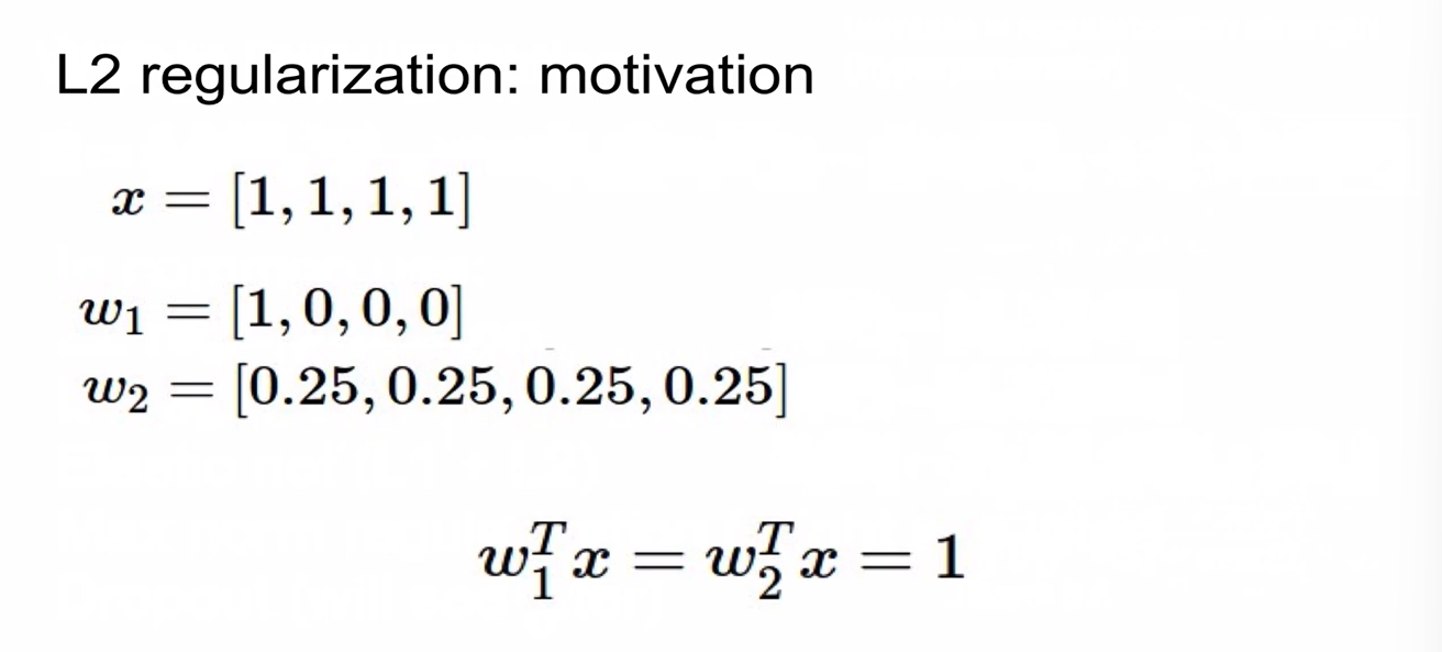
• L2 regularization: weight를 spread out해서 모든 input feature를 고려하도록 함.
  위 그림에서 w2가 더 좋은 weight임.

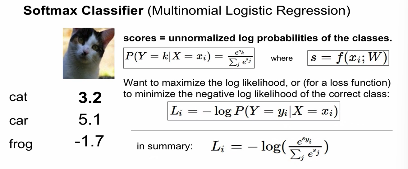
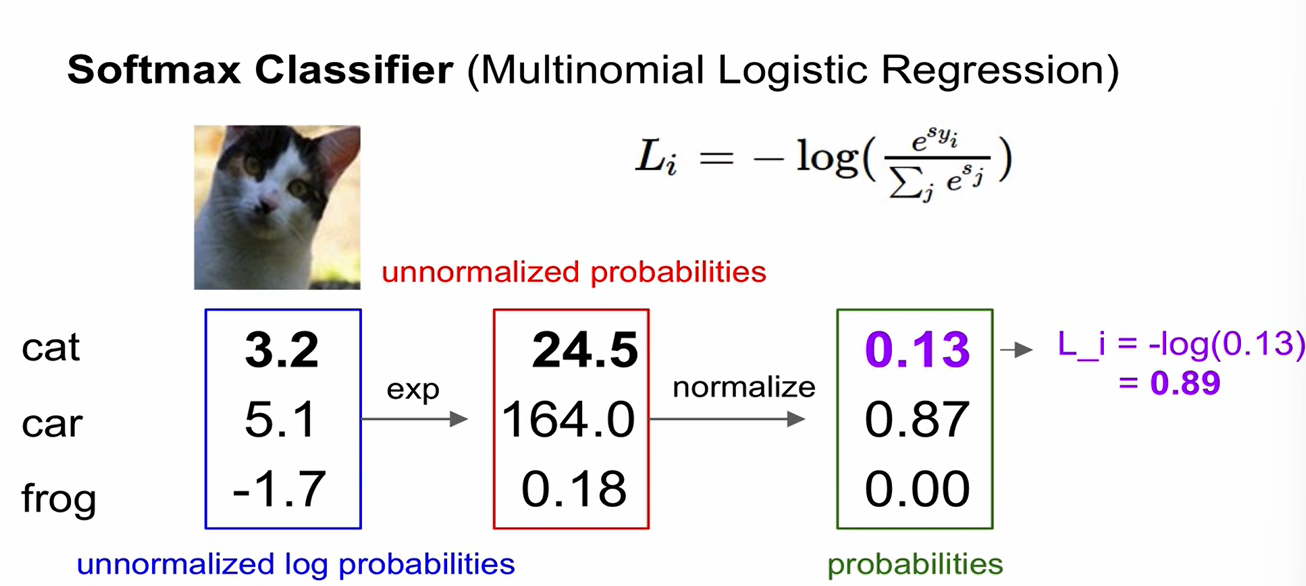
Softmax Classifier (Multinomial Logistic Regression)

• scores = unnormalized log probabilities of the classes
  

• 최솟값 = 0 (x=0) / 최댓값 = $\infty$
• Sanity check:
  initial loss (when W is small num so all s~=0)
  = $-log(1/class의 개수)$

• datapoint의 값이 약간 변하게 되면?

  • SVM: safety margin(1)을 더해줘서 robust. loss에 변화 없음. 둔감함
  • Softmax: 모든 인자를 고려하기 때문에 매우 sensitive한 모델임.

  

• Regularization loss의 경우, 데이터의 함수가 아니라 Weight만의 함수임. Weight에만 영향을 받음.

  Optimization

  • Random Search (X)

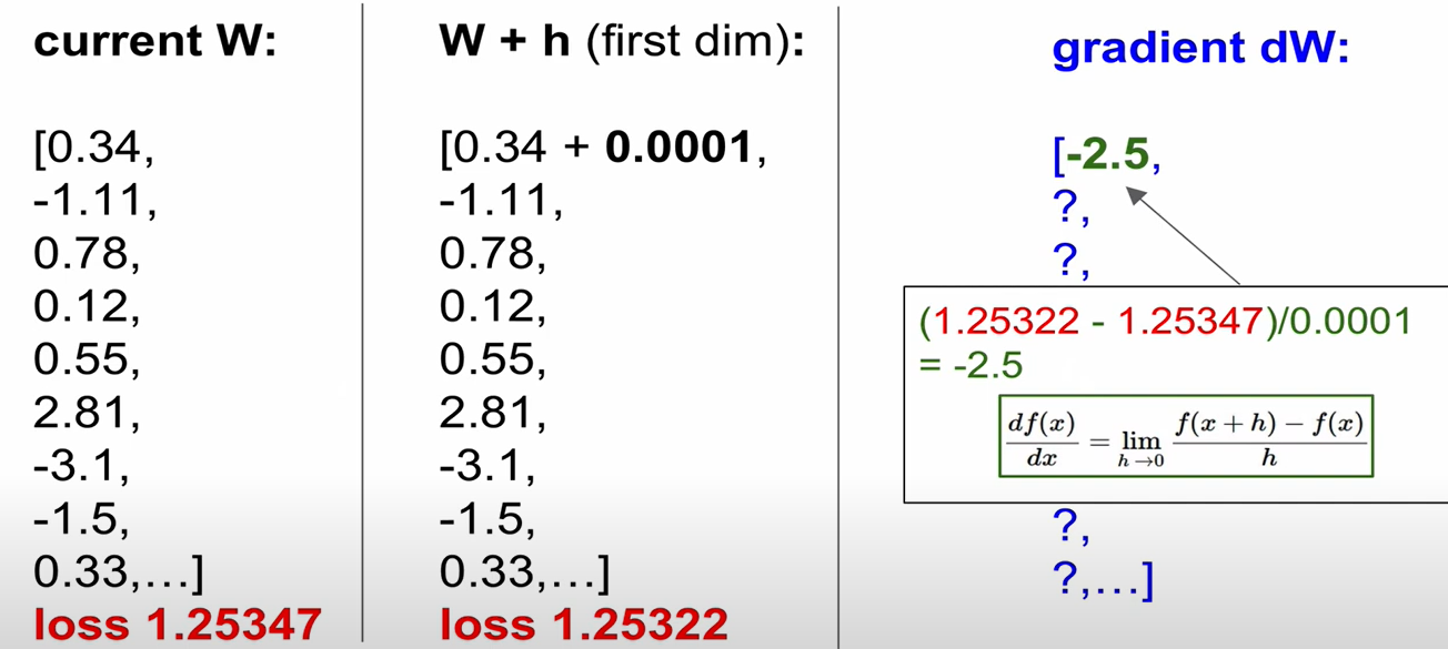
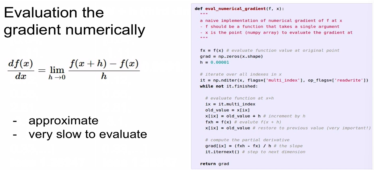
  • Follow the Scope - (1) numerical gradient: 하나하나 계산해서 미분을 구함

  

  Gradient 음수 -> downward / 양수 -> upward

  

• (2) analytic gradient: 미분해서 gradient를 구함

• Gradient Check: 항상 analytic gradient를 사용하지만, numerical gradient를 사용해서 맞게 구현되었는지 확인해야 함.

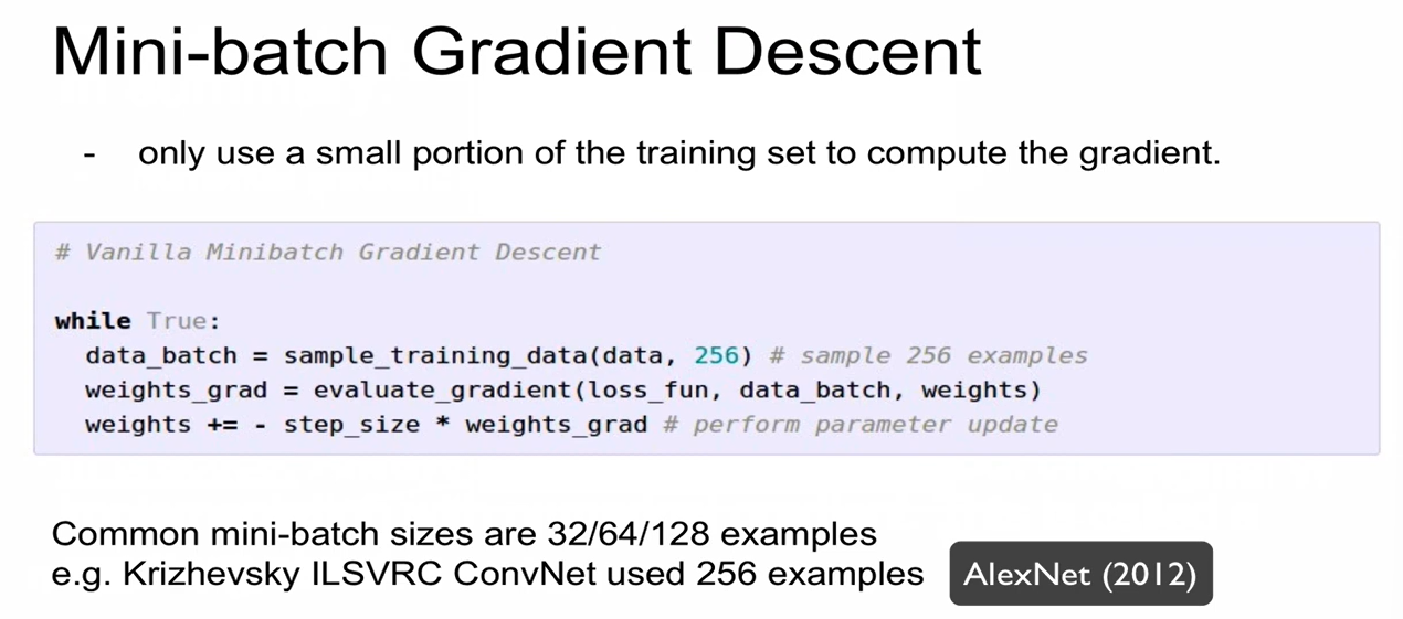
• Full batch graident descent: 모든 training set을 사용함
• Mini batch gradient descent: training set 중 일부만 활용하여 gradient를 계산함
  

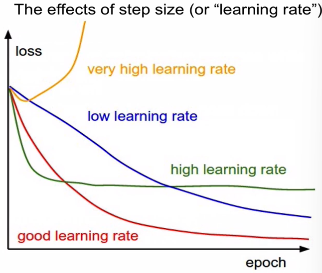
• Decay: learning rate를 높게 잡았다가 낮추는 것

ex) other fomulas: momentum, adagrad, rmsprop, adam ...

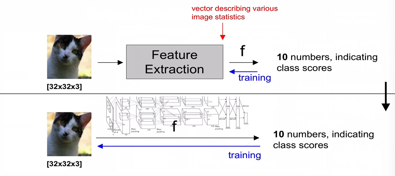
+) deep learning을 사용하지 않고 image feature를 추출하는 방식
(1) color (hue) histogram
(2) hog/sift features (edge의 orientation을 feature로 추출)
(3) bag of words: visual word vector -> learn k means centorids vocabulary of visual words -> feature 추출

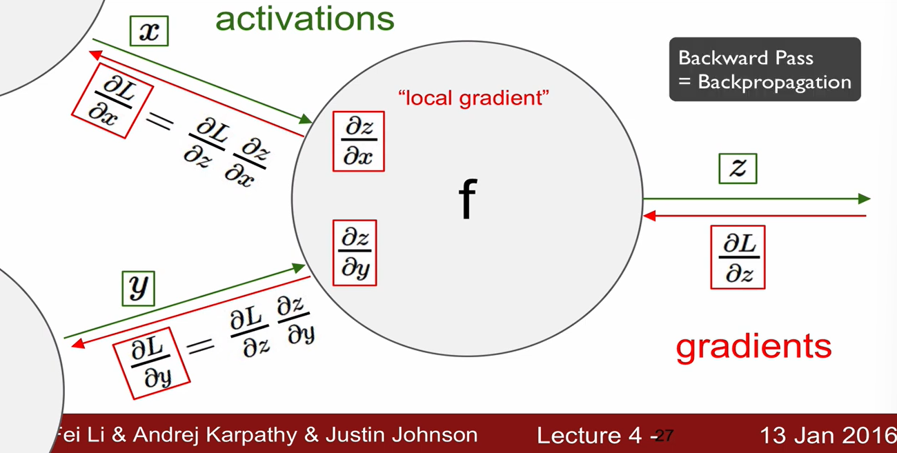
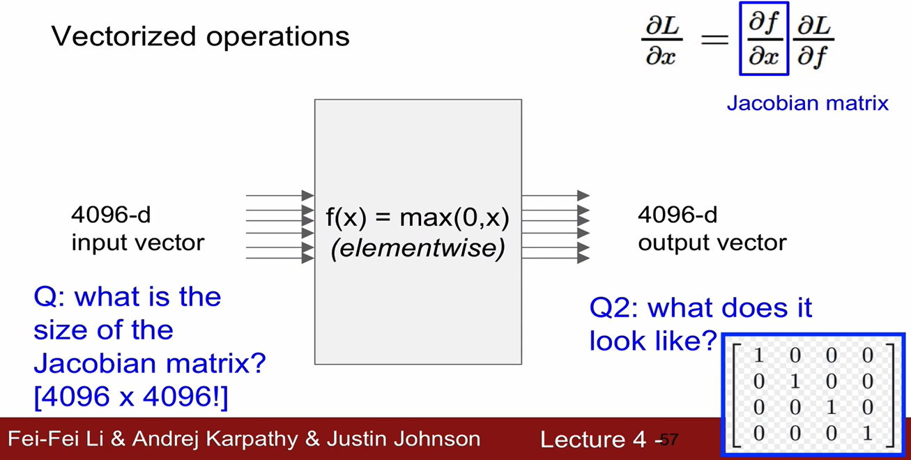
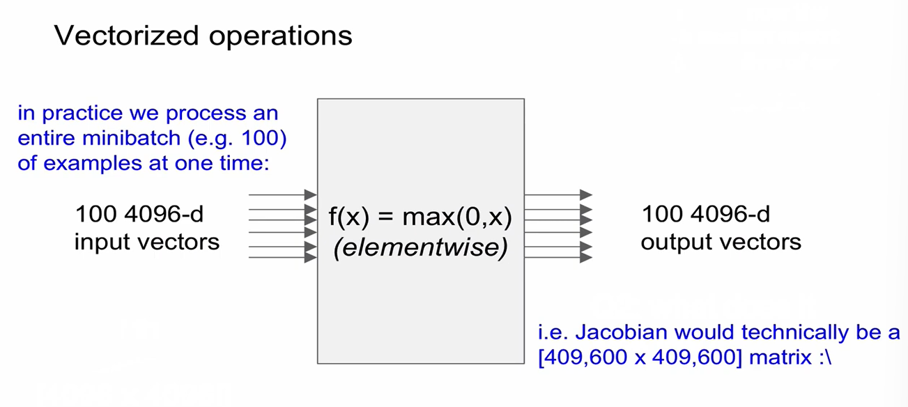
Back Propagation

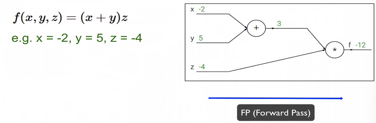
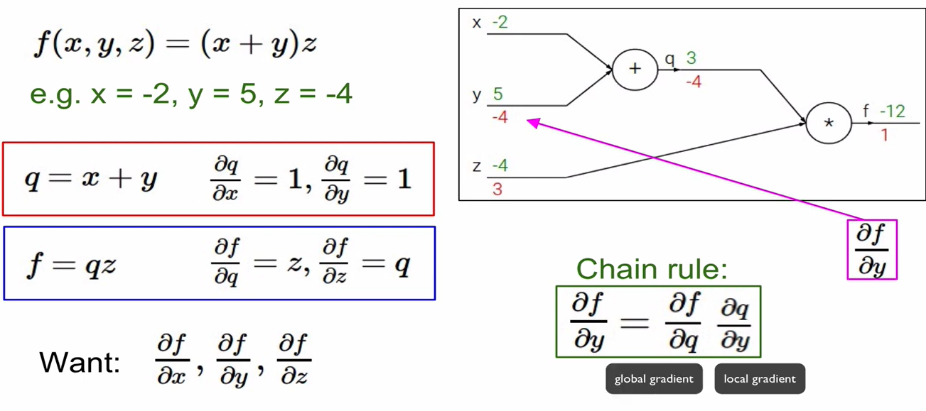
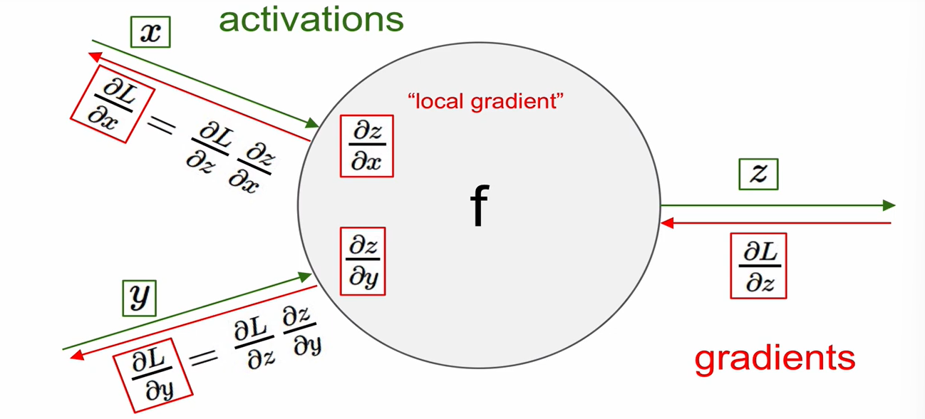
• x에 대한 gradient를 구할 때, x에 대한 미분식은 local gradient가 되고, 만약 x에 대한 미분항이 아닌 경우 이를 global gradient라 한다.
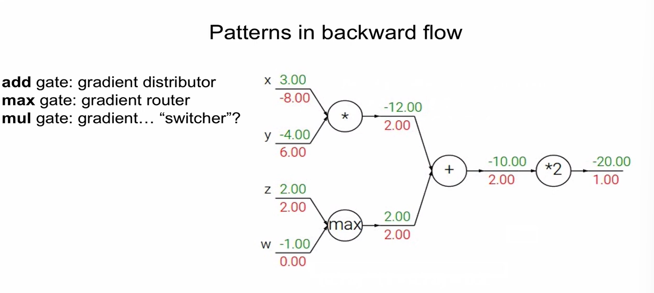
• 덧셈으로 연결된 경우 gradient 값은 항상 1이며, 곱셈으로 연결된 경우 gradient 값은 항상 반대(곱해진 것)의 값임.
  $q=x+y$ --> $\frac{\partial q}{\partial x} = 1, \frac{\partial q}{\partial y} = 1$
  $f=qz$ --> $\frac{\partial f}{\partial q} = z, \frac{\partial f}{\partial z} = q$
• 즉, local gradient는 forward pass 시에 구해서 memory에 저장해둠.
• global gradient는 backward pass 시만 구할 수 있음.
  -> local graident와 global graident를 곱해서 gradient를 얻을 수 있음.
  backward pass 시에 최종적으로 chaining이 일어남.

• z가 여러 개의 노드로 이루어진 경우에는 다 더해주면 됨.

• 예시
  

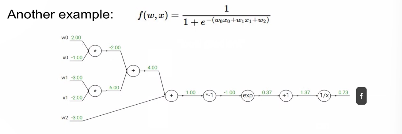
• 구하고자 하는 것: input(w0,x0,w1,x1,w2) 각각에 대한 loss에 대한 영향력
  즉, $\frac{\partial f}{\partial w0},\frac{\partial f}{\partial x0}, \frac{\partial f}{\partial w1}, \frac{\partial f}{\partial x1}, \frac{\partial f}{\partial w2}$의 값
• 초록색: 실제 변수 값, local gradient ($\frac{\partial f}{\partial x}$에 값을 넣어서 구해줌
• 빨간색: global gradient
• 더하기 연산 = gradient distributor (gradient를 동일한 값으로 전파해줌)
  

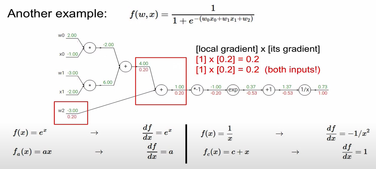
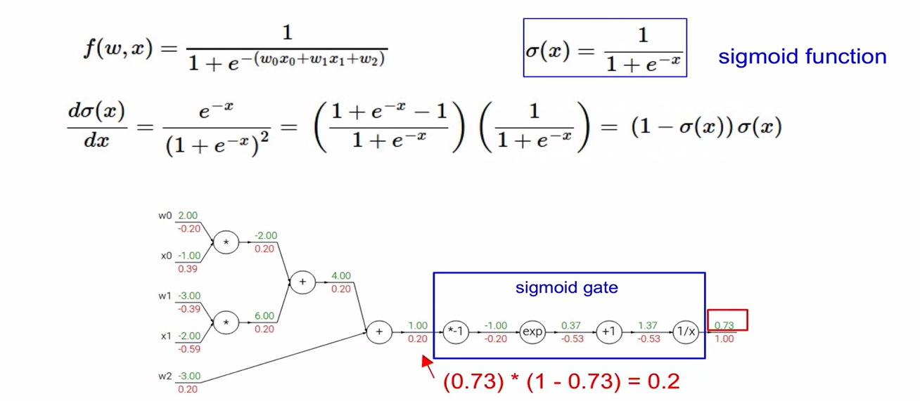
• sigmoid 함수
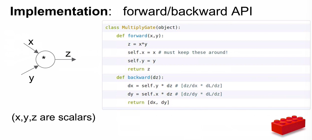
  • forward pass: $1/(1+exp(-x))$
  • backward pass: $(1-\sigma(x))(\sigma(x))$ (미분한 형태)

** assignment하기! forward pass & backward pass 구현하기

32:44부터 듣기 (neural network)