Introduction to Causal Inference: Lecture 4 Backdoor Adjustment & Structural Causal Models

Brady Neal의 introduction to causal inference 리뷰입니다.
youtube: https://www.youtube.com/watch?v=dB8r4Afmobo&list=PLoazKTcS0Rzb6bb9L508cyJ1z-U9iWkA0&index=27
material: https://www.bradyneal.com/causal-inference-course
My article will be uploaded to https://www.notion.so/GNN_YYK-0303f11d4fa0433792562333dea173a3.

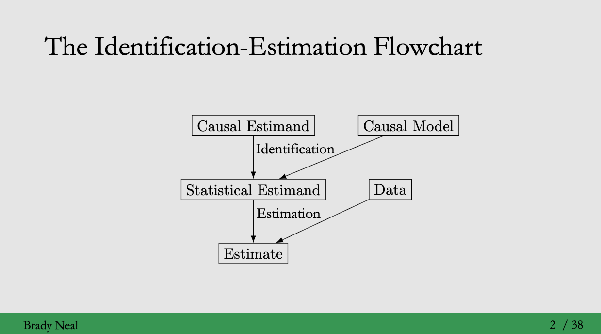
Identification: the process of moving from a causal estimand to a statistical estimand (Lectrue 2 참고)

Identification을 위해서는 causal model이 필요합니다.

지난 3강에서 causal models을 위한 graphical models에 대해 공부했습니다. 이번 강의에서는 how to identify causal quantities와 how to formalize causal models을 다룹니다.

Sub-project on causal inference (Yong-min shin, GNN-YYK, Lecture 2)

The do-operator

강의에서 두 가지 텀, conditioning과 intervening이 등장합니다.

• Conditioning $T=t$
  모집단에서 treatment $t$를 시행한 부분집합으로 범위를 제한하는 것과 같음.
• intervention
  모집단을 취하고 모두에게 treatment $t$를 시행한 것

이를 도식화 하면 다음과 같습니다.

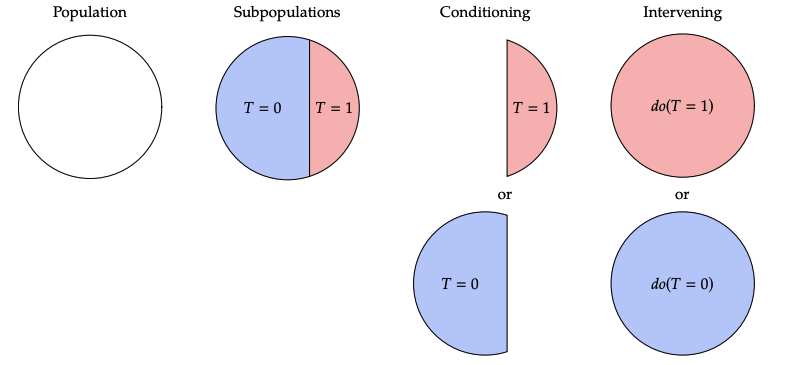
Interventional distribution $P(Y|do(T=t))$는 obsevational distribution $P(Y)$와 다릅니다.
$P(Y)$ 혹은 $P(Y,T,X)$와 같은 obsevational distribution은 do operator를 갖지 않기 때문에, 어떤 실험을 수행하지 않고도 데이터를 관찰할 수 있습니다. 따라서 $P(Y,T,X)$에서 데이터를 obsevational data라고 부릅니다.

위에서 identification 정의를 이해하셨다면, do operator를 가진 표현 $Q$에서 do 를 제거할 수 있다면 $Q$는 identifiable 되었다!는 것을 이해할 수 있을 것입니다.

그렇다면, do operator는 무엇을 의미할까요? 일반적으로 do 는 확률 $P$에서 conditioning bar 뒤에 나타납니다. 이때는 intervention do($t$) 가 발생한 다음을 의미하는 것으로, 즉 post-intervention 을 의미합니다.

예를 들어, $E[Y|do(t), Z=z]$에서 $Z=z$인 subpopulation에서(conditioning), 모두에게 treatment $t$를 시행한 후(intervening)의 기대되는 값을 의미합니다.
그렇다면 $E[Y|Z=z]$는? 단순히 개인이 일반적으로 treatment $T$를 받은 (pre-intervention) 집단에서 기대되는 값을 의미합니다.

Main assumption: modularity

Modularity를 이해하기 위해서는 causal mechanism 에 대해 이해해야 합니다. Causal mechnism을 아주 간단히 표현한다면, conditional distribution $P(x_i | pa_i)$ 입니다.

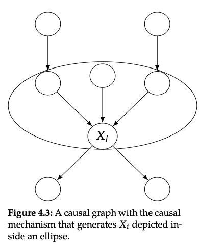
Causal identification 결과를 얻기 위해서 중요한 가정은 "interventions are local" 입니다. 좀 더 자세하게 말하자면, 변수 $X_i$에 intervening하면, 오직 $X_i$의 causal mechanism만 변하게 됩니다. 즉 다른 변수들을 만드는 causal mechanisms은 변하지 않게 됩니다. 이런 의미로 causal mechnisms은 modular입니다.

일반적으로 modular property를 independent mechnisms, autonomy 혹은 invariance라고도 부릅니다.

Assumption 4.1 (Modularity Independent Mechnisms) If we intervene on a set of nodes $S \subseteq [n]$, setting them to constants, then for all $i$, we have the following:
1. if $i \notin S$, then $P(x_i|pa_i)$ remains unchanged.
2. if $i \in S$, then $P(x_i|pa_i)=1 \; if x_i$ is the value that $X_i$ was set to by the intervention; otherwise, $P(x_i|pa_i)=0$.

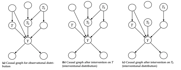
Modularity assumption은 하나의 그래프에서 서로 다른 interventional distribution을 만들 수 있게 해줍니다. 예를 들어 $P(Y), P(Y|do(T=t)), P(Y|do(T=t')), P(Y|do(T_2=t_2))$는 서로 연관되지 않은 완전히 다른 분포입니다. 즉 intervention을 통해 각 분포가 자기 자신만의 그래프를 만든 것입니다.

interventional distributions의 causal graph는 obsevational joint distribution(original graph)에서 사용된 것과 같지만, intervened node(s)의 엣지가 제거된 형태입니다. 이는 intervened factor의 확률이 1이기 때문에, 관련 factor들을 무시한다고 보면 됩니다. 또 다른 관점으로는 intervened node가 constant로 설정되었기 때문에 더이상 다른 변수에 의존하지 않는다라고 볼 수 있습니다.

엣지가 제거된 그래프를 manipulated graph 라고 합니다.

Modularity assumption이 위반된다라는 것은 어떤 것을 의미할까요?

$X_i$를 intervene 했을 때, 이것이 다른 노드 $X_j$를 변하게 하는 경우입니다. 즉 intervention on $X_i$가 $P(x_j|pa_j)$를 변화시키는 것입니다. (intervention is not local to the node you intervene on; the causal mechnisms are not modular)

Backdoor adjustment

Backdoor path란 노드 $T$에서 노드 $Y$까지 nondirected unblocked path(즉 $T$로 가는 backdoor edge가 존재함)를 의미합니다. 그리고 conditioning을 통해 이것을 block할 수 있다면 causal quntity를 구할 수 있을 것입니다.

만약 $T$에 intervene을 해준 manipulated graph가 있다면 해당 그래프에는 T의 backdoor edge가 존재하지 않을 것이고, 이는 $T$에서 $Y$까지 흐르는 모든 association은 purely causal일 것입니다.

Definition 4.1 (Backdoor Criterion) A set of variables $W$ satisfies the backddor criterion relative to $T$ and $Y$ if the following are true:
1. $W$ blocks all backdoor paths from $T$ to $Y$.
2. $W$ does not contain any descendants of $T$.

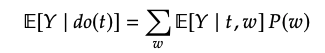
Backdoor criterion을 만족한다는 것은 $W$를 sufficient adjustment set으로 만드는 것입니다. $W$는 앞의 예제에서 등장했던 $X$라고 생각하면 됩니다. 이 예에서는 오직 하나의 path만 존재했기 때문에 단순히 $X$만으로도 충분히 block할 수 있었습니다.

proof에 $W$를 도입하기 위해 변수를 conditioning해주고 marginalizing을 해주게 됩니다.

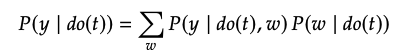
주어진 $W$가 Backdoor criterion을 만족한다면, modularity 가정을 통해 아래가 가능합니다.

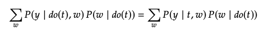
위의 식을 보면, 여전히 식에 do 가 존재합니다. 그러나 여기서 $P(w|do(t))=P(w)$가 됩니다. Manipulated graph에서 $T$로 들어오는 엣지가 없기 때문에 어떠한 $W$와 $T$사이의 path도 존재하지 않습니다.
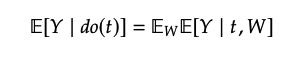
따라서 위의 식은 아래와 같이 정리됩니다.

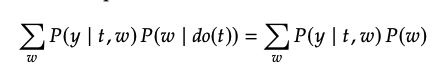
이것이 backdoor adjustment 입니다.

Theorem 4.2 (Backdoor Adjustment) Given the modulrarity assumption, that $W$ satifies the backdoor criterion, and positivity(Assumption 2.3), we can idenify the causal effect of $T$ on $Y$:
$P(y|do(t))=\sum_w P(y|t,w)P(w)$

Relation to d-separation $W$가 manipulated graph $T$와 $Y$를 d-separated 하는 경우 backdoor adjustment를 쓸 수 있습니다. 또한 $W$를 conditioning 함으로써 pure causal association 할 수 있습니다.

Q) How does this backdoor adjustment relate to the adjustment formula we saw in the potential outcomes lecture?

Adjustment formula

위는 아래의 backdoor adjusment로 유도됩니다.

($w$가 discrete이 아닌 경우, integral)

$\because(Y(1), Y(0)) \perp \!\!\! \perp T | W$

Structural causal models

Structural Equations

수학에서 쓰는 equals sign(=)과는 다르게, causation에서는 symmetric 성질이 성립하지 않습니다. 즉 A가 B의 cause라고 한다면 A의 변화는 B의 변화를 초래하지만, B의 변화가 A의 변화를 초래하지는 않습니다.
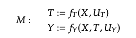
structural equation $B:=f(A)$
(=가 아닌 :=를 쓴 것을 유의!)

그러나, 여기서 $A$와 $B$의 mapping이 deterministic하기 때문에, 이를 probabilistic으로 만들기 위한 B의 unknown causes에 대한 여지를 남기게 됩니다.
$B:=f(A,U)$

endogenous variables: 우리가 모델링을 하려는 structural equation의 variable. 즉 causal graph에서 부모 노드를 갖고 있음.
exogenous variables: causal graph에서 부모 노드가 없는 변수. 즉 이 노드의 causes를 모델링할 필요가 없음.

Definition 4.2 (Structural Causal Model (SCM)) A structural causal model is a tuple of the following sets:
1. A set of endogenous variables V
2. A set of expgenous variables U
3. A set of functions f, one to generate each endogenous variable as a function of other variables

Markovian vs. semi-Markovian vs. non-Markovian

Markovian: causal graph에 사이클이 없고(DAG), noise variables $U$가 독립인 경우
semi-Markovian: causal graph에 사이클이 없고(DAG), noise variables $U$가 독립이 아닌 경우
non-Markovian: 사이클이 있는 경우

Interventions

SCM에서는 intervention이 매우 간단합니다. $T$를 $T:=t$로 대체해주면 됩니다.

(여기서 $M$은 a single model의 모든 structural equation의 collection)

($M_t$임을 유의)

Definition 4.3 (The Law of Counterfactuals (and Interventions))
$Y_t(u)=Y_{M_t}(u)$

이는 SCM이 디테일하게 주어진다면 couterfactuals을 모두 계산할 수 있다는 것을 의미합니다. 그러나 이것은 불가능하기 때문에 큰 문제가 됩니다. 이 문제를 해결하기 위한 conterfactuals은 14장에서 다루고 있습니다.

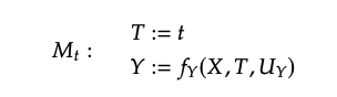
A complete example with estimation

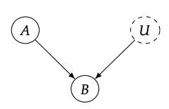
association quantity($E[Y|t]$)와 causal quantity($E[Y|do(t)]$)의 비교를 통해 association quantity의 bias를 알아보기 위해 toy example을 살펴봅시다.

$T:=\alpha_1 X$
$Y:=\beta T + \alpha_2 X$

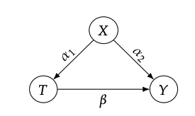
causal quantity($E[Y |do(t)]$)

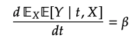
그림에서 볼 수 있듯이, $X$가 sufficient adjustment set이므로, $E[Y|do(t)]=E_xE[U|t,X]$ 입니다.

따라서,
$E_xE[U|t,X]=E_x[E[\beta T+\alpha_2 X | T=t, X]]=E_x[\beta t + \alpha_2 X]=\beta t + \alpha_2 E[X]$

causal effect를 얻기 위해 미분을 해주면,

association quantity ($E[Y|t]$)

$E[Y|T=t]=E[\beta T + \alpha_2 X|T=t]= \beta t +\alpha_2 E[X|T=t]=\beta T + {\alpha_2 \over \alpha_1}t$

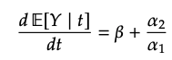
위 그림과 같이, confounding bias가 존재합니다.