VIT code (with attention matrix)

모듈 불러오기

%%capture
!pip install timm

import os
import matplotlib.pyplot as plt
import numpy as np
import PIL

import torch
import torch.nn.functional as F
import torchvision
import torchvision.transforms as T

from timm import create_model

## timm은 여러가지 computer vision모델들을 포함하고 있는 모듈이다. 

모델 선언 및 데이터 로드

## 모델 선언
model_name = "vit_base_patch16_224"
device = 'cuda' if torch.cuda.is_available() else 'cpu'
print("device = ", device) 
model = create_model(model_name, pretrained=True).to(device)
# timm의 장점으로 model 이름만 넣어주면 사전에 학습된 model을 생성할 수 있다.

## image transform 선언
여러 이미지가 들어오기 때문에 모델 input에 맞게 224,224로 맞춰주고 tensor화 시켜주고
정규화를 진행한다.
IMG_SIZE = (224, 224)
NORMALIZE_MEAN = (0.5, 0.5, 0.5)
NORMALIZE_STD = (0.5, 0.5, 0.5)
transforms = [
              T.Resize(IMG_SIZE),
              T.ToTensor(),
              T.Normalize(NORMALIZE_MEAN, NORMALIZE_STD),
              ]

transforms = T.Compose(transforms)

## 데이터 로드
## 외부 웹페이지에서 데이터를 다운 받는 !wget을 이용해서 데이터 다운 받기
%%capture
# ImageNet Labels(클래스)
!wget https://storage.googleapis.com/bit_models/ilsvrc2012_wordnet_lemmas.txt
imagenet_labels = dict(enumerate(open('ilsvrc2012_wordnet_lemmas.txt')))

# Demo Image
!wget 이미지가 있는 주소 넣기
img = PIL.Image.open('santorini.png')
img_tensor = transforms(img).unsqueeze(0) .to(device)

이미지를 패치로 나누기

직접 짜보기

import torch.nn as nn

class PatchEmbed(nn.Module):
    def __init__(self, img_size=224, patch_size=16, in_chans=3, embed_dim=768):
        super(PatchEmbed, self).__init__()

        self.img_size=img_size
        self.patch_size=patch_size
        self.in_chans=in_chans
        self.embed_dim=embed_dim
        self.grid_size=int(img_size/patch_size)
        self.patch_num=int((img_size/patch_size))**2

		# 3x16x16 필터를 768개를 만들어 input data 1x3x224x224가 들어오면
        # stride 16을 이용해 필터를 통과하면
        # 1x768x14x14 차원을 가진 output이 나온다.
        self.proj = nn.Conv2d(in_chans,embed_dim,kernel_size=patch_size,stride=patch_size)

	
    def forward(self, x):
    
        x=self.proj(x)
        # 이미지 패치를 일렬로 배치하기 위해 flatten을 사용하면 1x768x196 차원이 된다.
  		# flatten(2)는 2차원부터 끝까지를 일렬로 펼치겠다는 의미
        x=x.flatten(2) 
        x=x.transpose(1,2)
        # dim=2와 dim=1를 바꾸면 1x196x768이 된다.

        return x
        
        # 이렇게 바꾸면 이제 196은 각각의 이미지 토큰을 의미하고
        # 각각의 토큰의 임베딩 벡터들이 768 차원으로 만들어진 것이다.

model 함수 사용하기

## patch_embed를 사용하면 된다.
patches = model.patch_embed(img_tensor)  # patch embedding convolution

나누어진 패치 잘 나누어졌나 시각화 해보기

# 패치로 나누어진 image 시각화
fig = plt.figure(figsize=(8, 8))
fig.suptitle("Visualization of Patches", fontsize=24)
fig.add_subplot()
img = np.asarray(img) # 시각화를 위해 numpy로 변환
for i in range(0, 196):
    x = i % 14
    y = i // 14
    patch = img[y*16:(y+1)*16, x*16:(x+1)*16]
    ax = fig.add_subplot(14, 14, i+1)
    ax.axes.get_xaxis().set_visible(False)
    ax.axes.get_yaxis().set_visible(False)
    ax.imshow(patch)
    
# PyTorch의 텐서는 일반적으로 (C, H, W) 형식(채널, 높이, 너비)으로 저장됩니다. 
# 반면에, 시각화 라이브러리들은 보통 (H, W, C) 형식(높이, 너비, 채널)을 기대합니다. 그래서 바꾸어 준다.

position embedding

# 이 모델 자체가 224x224를 16x16패치로 이미 학습되어있어서 바로 불러올 수 있다.
pos_embed = model.pos_embed

# 1x197x768 차원을 갖는데 196에서 1이 증가한 것을 알 수 있다 이것은 cls토큰까지 넣은 것을 고려한 것이다.

transformer input 생성

# cls 토큰 생성
cls=model.cls_token

# 패치 생성
patches=model.patch_embed(img_tensor)

# 토큰과 패치 합치기
patches=torch.cat((cls,patches),1)
# 이렇게 하면 1x197x768이 된다.

# 포지셔닝 임베팅 벡터 생성
pos_embed=model.pos_embed

# 두 벡터를 더해 input 생성
transformer_input = torch.add(patches,pos_embed)

VIT attention matrix

attention matrix visualization

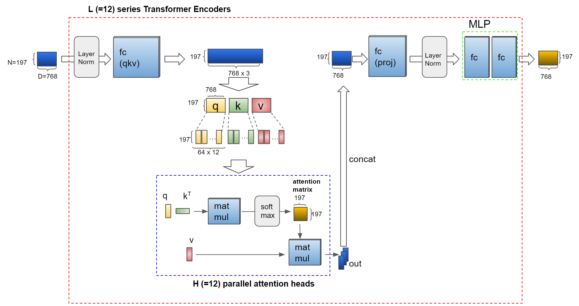
VIT의 multi-head는 12개로 구성되어 있다.
이것에 맞춰서 encode 코드를 구현하여 attention matrix를 시각화 해보자

# Input의 dimension을 expand하기 위해 fc layer 적용
# query,key,value가 필요함으로 768 * 3 정도가 필요하다. 그래서 확장시켜주어야 한다.
transformer_input_expanded = attention.qkv(transformer_input)[0]



# Multi-head attantion을 위해 qkv를 여러개의 q, k, v vector들로 나눕니다.
qkv = transformer_input_expanded.reshape(197, 3, 12, 64)  # (N=197, (qkv), H=12, D/H=64)
print("split qkv : ", qkv.shape)
q = qkv[:, 0].permute(1, 0, 2)  # (H=12, N=197, D/H=64)
k = qkv[:, 1].permute(1, 0, 2)  # (H=12, N=197, D/H=64)
kT = k.permute(0, 2, 1)  # (H=12, D/H=64, N=197)


# Attention Matrix
attention_matrix =torch.matmul(q,kT)
# 12헤드마다 197x197 attention matrix가 만들어 진다.

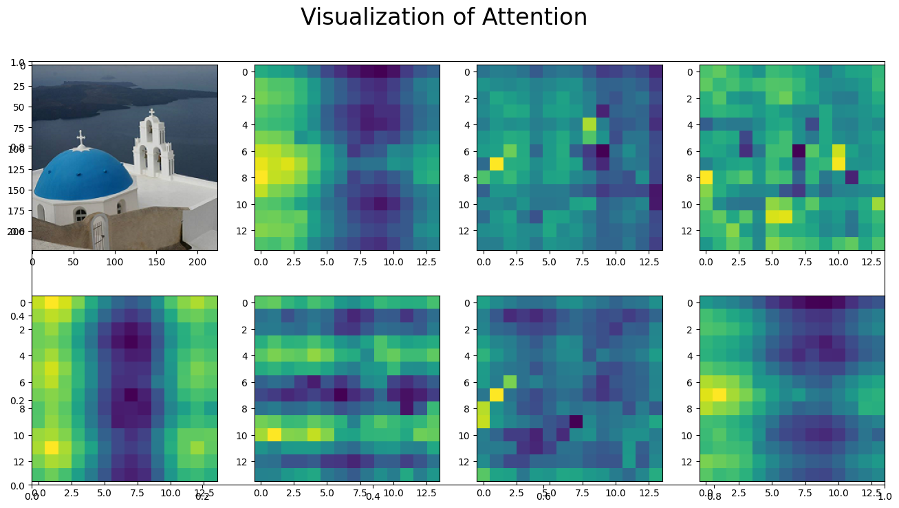
# Attention matrix 시각화
fig = plt.figure(figsize=(16, 8))
fig.suptitle("Visualization of Attention", fontsize=24)
fig.add_subplot()
img = np.asarray(img)
ax = fig.add_subplot(2, 4, 1)
ax.imshow(img)
for i in range(7):  # 0-7번째 헤드들의 100번째 줄(row)의 attention matrix 시각화
    attn_heatmap = attention_matrix[i, 100, 1:].reshape((14, 14)).detach().cpu().numpy()
    ax = fig.add_subplot(2, 4, i+2)
    ax.imshow(attn_heatmap)
# 이렇게 하면 100번째 이미지 토큰이 헤드별로 주위의 이미지 토큰을 보았을 때 attention 시각화가 나오게 된다.

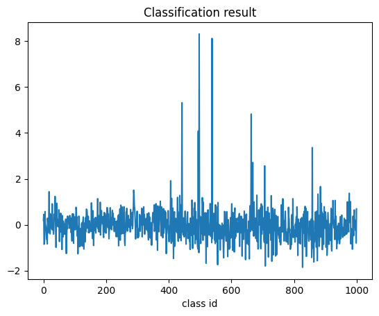
MLP Head visualization

#Transformer output vector의 0번째값은 class token input에 대응됩니다. 
1000-dimension의 classification 결과가 전체 파이프라인의 output입니다

result = model.head(transformer_output)
result_label_id = int(torch.argmax(result))
plt.plot(result.detach().cpu().numpy()[0])

print("Inference result : id = {}, label name = {}".format(
    result_label_id, imagenet_labels[result_label_id]))