PCA, t-SNE, MDS, Isomap 을 이용한 2,3차원 도형 차원 축소

Level2 멘토링 첫번째 과제

차원축소 감잡기

1-dimensional manifold in R^2: 원,
2-dimensional manifolds in R^3: 구, 토러스, 원기둥

• 각 도형의 매개변수식을 위키피디아에서 검색.
• 넘파이로 각 도형의 포인트들을 랜덤 샘플링해서 저장.
• 높이를 기준으로 각 포인트의 색을 지정.
• PCA, MDS, ISOMAP, LDA, tSNE로 매개변수 차원으로 축소한 뒤 지정된 색에 따라서 시각화.
• 팀원들과 각 차원 축소법이 어떤 특징을 가지고 있는지 토의.

---

import numpy as np
import matplotlib.pyplot as plt

from sklearn.decomposition import PCA, LatentDirichletAllocation
from sklearn.manifold import Isomap, TSNE, MDS

1. 원 (PCA)

R = 1
n = 64
t = np.linspace(0, 2*np.pi, n+1)
x = R * np.cos(t)
y = R * np.sin(t)
idx = [i for i in range(len(x))]
a = np.random.choice(idx, int(len(x) * 0.5), replace=False)
z = [i for i in range(len(a))]
plt.axis('equal')
plt.grid()
plt.title('original')
plt.scatter(x[a], y[a], c=y[a])
plt.show()
#
z = []
for i, j in zip(x,y):
    k = [i, j]
    z.append(k)
z = np.array(z)
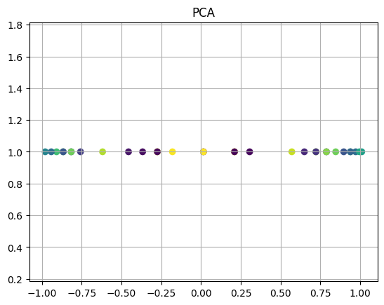
# PCA
pca = PCA(n_components = 1)
pca_done = pca.fit_transform(z)
plt.axis('equal')
plt.grid()
plt.title('PCA')
plt.scatter(np.array(pca_done[a]), [1 for i in range(len(a))], c=y[a])
plt.show()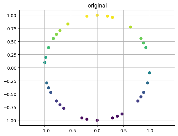

2. 원기둥

1) PCA

from mpl_toolkits.mplot3d import Axes3D
import numpy as np
import matplotlib.pyplot as plt
import random

"""
equation for a circle

x  =  h + r cosθ
y  =  k + r sinθ

where h and k are the co-ordinates of the center

0 <= θ <= 360
"""
fig = plt.figure()
ax = fig.add_subplot(111, projection='3d')

theta = np.linspace(0, 2 * np.pi, 201)
radius = 1

x = np.linspace(0, 50, 100)
# print(x)
thetas, xs = np.meshgrid(theta, x)
# print(xs)
c = xs
y = radius * np.cos(thetas)
z = radius * np.sin(thetas)

ax.scatter(y, z, xs, c=c, alpha=0.2)

ax.set_xticks([-radius, 0, radius])
ax.set_yticks([-radius, 0, radius])
ax.set_zticks([0, 50])

plt.show()

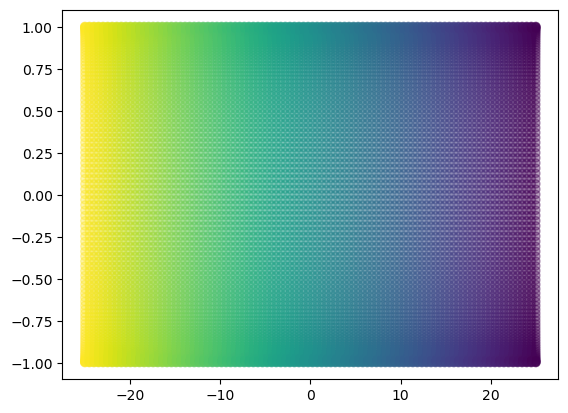
xs_r = xs.reshape(-1,1)
y_r = y.reshape(-1,1)
z_r = z.reshape(-1,1)
c_r = c.reshape(-1,1)

concat = np.concatenate((y_r,z_r,xs_r),axis=1)

pca = PCA(n_components=2)
concat_pca = pca.fit_transform(concat)

# 1d array
t = np.array([0]*20100)
t = t.reshape(-1,1)

plt.scatter(concat_pca[:,0], concat_pca[:,1], c=xs_r, alpha = 0.2);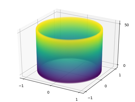

2) t-SNE

from sklearn.manifold import TSNE,Isomap

model = TSNE(learning_rate=100)
transformed = model.fit_transform(concat)

xs = transformed[:,0]
ys = transformed[:,1]

plt.scatter(xs,ys,c=c_r)
plt.show()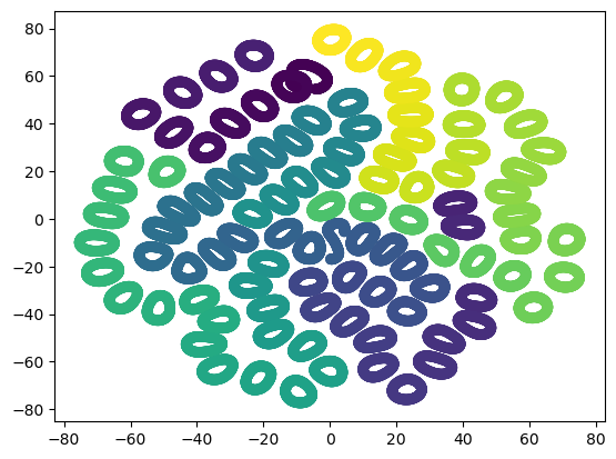

3) Isomap

isomap = Isomap(n_components=2)
concat_isomap = isomap.fit_transform(concat)
fig = plt.figure()
plt.title('isomap')
plt.scatter(concat_isomap[:,0], concat_isomap[:,1],c=z)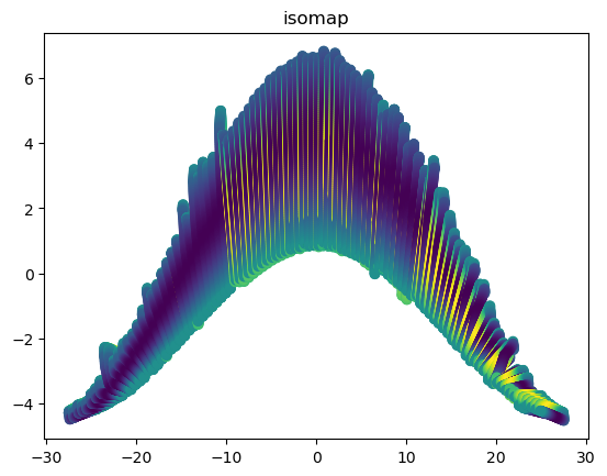

3. 구

PCA

import numpy as np
import matplotlib.pyplot as plt

n = 1000
r = 1

ang1 = np.random.normal(0, 2*np.pi, n)
ang2 = np.random.normal(0, np.pi, n)

x = r*np.cos(ang1)*np.cos(ang2)
y = r*np.sin(ang1)*np.cos(ang2)
z = r*np.sin(ang2)


fig = plt.figure()
ax = plt.axes(projection='3d')
ax.scatter(x, y, z, 
           c=(x+y+z))


ax.set_zlim([-1,1])

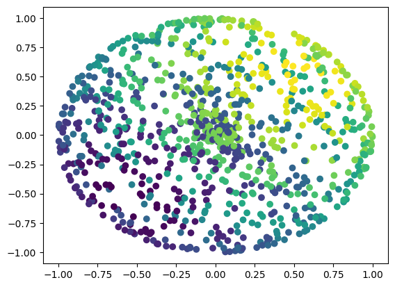
X = np.array([(a,b,c) for a,b,c in zip(x,y,z)])

pca = PCA(n_components=2)
sph_pca = pca.fit_transform(X)
sph_pca

fig = plt.figure()
ax = plt.axes()

ax.scatter(X[:,0], X[:,1], c=(x+y+z))
plt.show()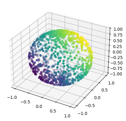

4. 토러스

1) PCA

fig = plt.figure(figsize=(plt.figaspect(0.7)))
ax = fig.add_subplot(111, projection='3d')
n = 64
U = (np.random.random(n ** 2) * 2*np.pi).reshape(n,n)
V = (np.random.random(n ** 2) * 2*np.pi).reshape(n,n)
a = 3
b = 0.5
X = (a + b * np.cos(V)) * np.cos(U)
Y = (a + b * np.cos(V)) * np.sin(U)
Z = b * np.sin(V)
W = Z.reshape(-1)
surf = ax.scatter(X,Y,Z, c=W, cmap='Greens',
        linewidth=0.01, antialiased=False, alpha = 0.5)
ax.set_zlim3d(-2.01, 2.01)
fig.colorbar(surf, shrink=0.5, aspect=10)
plt.show()
lst = []
for x,y,z,w in zip(X.reshape(-1),Y.reshape(-1),Z.reshape(-1), W.reshape(-1)):
    lst.append((x,y,z,w))
lst = np.array(lst)
X = lst[:, :-1]
y = lst[:, -1]
pca = PCA(n_components=2)
pca_X = pca.fit_transform(X)
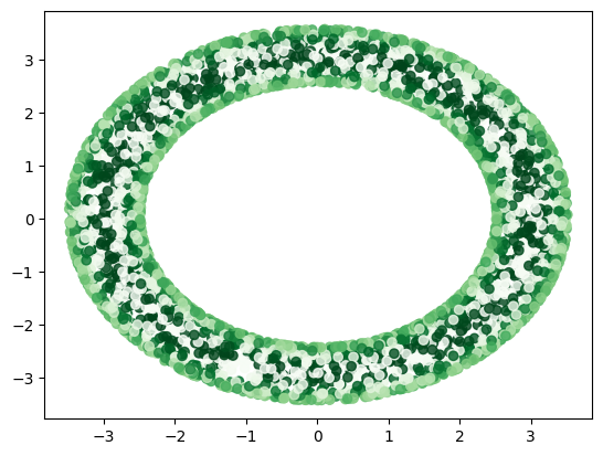
plt.scatter(pca_X[:, 0], pca_X[:, 1], c=y, cmap='Greens', alpha=0.8);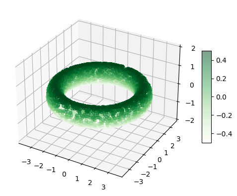

2) t-SNE

tsne = TSNE(n_components=2)
tsne_X = tsne.fit_transform(X)
tsne_X
plt.scatter(tsne_X[:, 0], tsne_X[:, 1], c=y, cmap='Greens', alpha=0.8);
plt.show()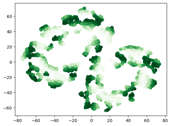

3) MDS

mds = MDS(n_components=2, verbose=1, max_iter=10)
mds_X = mds.fit_transform(X)
mds_X
plt.scatter(mds_X[:, 0], mds_X[:, 1], c=y, cmap='Greens')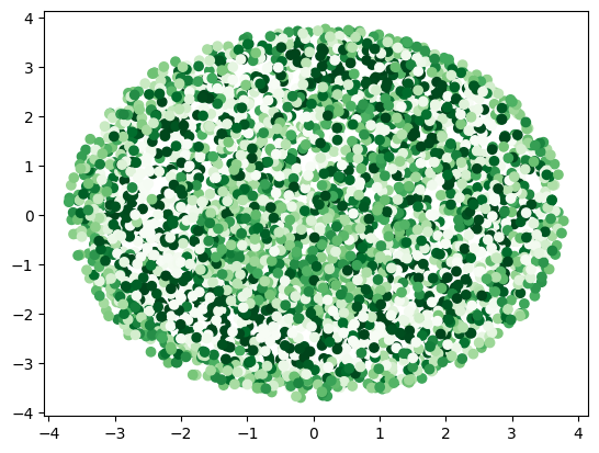

4) Isomap

iso = Isomap(n_components=2)
iso_X = iso.fit_transform(X)
iso_X
plt.scatter(iso_X[:, 0], iso_X[:, 1], c=y, cmap='Greens')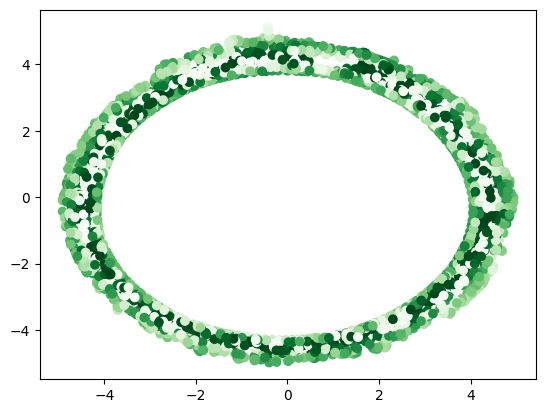

---

그림을 확인해보면 알겠지만, 도형의 높이 별로 다른 색을 지정해 차원축소를 하면 어떤식으로 점이 옮겨지는지, 투영되는지에 대해 감을 잡는 실습과제였다고 생각한다.

처음에는 어렵고 어떻게 해야할지 막막한 감이 있었지만 팀원들과 함께 문제를 해결 하다보니 재밌었고, 특히 PCA의 경우 어떤 관점에서 바라보기 때문에 데이터의 차원이 어떻게 축소되는지 간략하게나마 감을 잡을 수 있어서 좋았다