Logistic Regression
- 분류에 사용
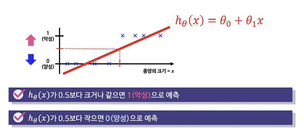
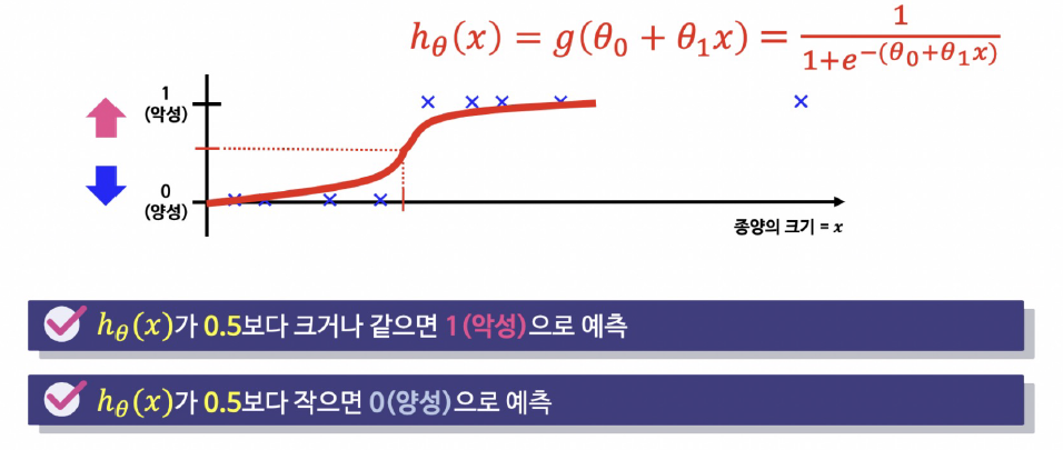
종양 크기 (x축)를 가지고 양성/악성을 판단하는 문제가 있다고 가정할때, 선형 회귀로 접근하면 정확히 분류하기 어려움.
분류 문제는 0/1로 예측해야 하나, 선형회귀를 적용하면 예측값은 0보다 작거나 1보다 큰 값을 가질 수 있다.
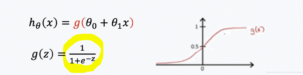
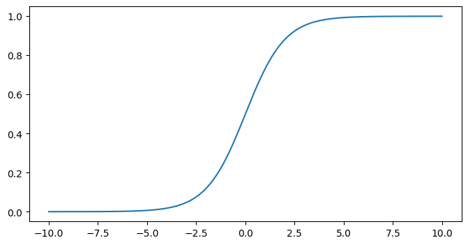
항상 0에서 1 사이 값을 가지도록 시그모이드 함수를 적용
import numpy as np

z = np.arange(-10, 10, 0.01)
g = 1 / (1+np.exp(-z))
import matplotlib.pyplot as plt
%matplotlib inline
plt.figure(figsize=(8,4))
plt.plot(z,g);
plt.figure(figsize=(8,4))
ax = plt.gca() #설정값 변경할 수 있음.
ax.plot(z,g)
ax.spines['left'].set_position('zero')  #위그래프의 좌측 축을 0 위치로 가져오는 옵션
ax.spines['bottom'].set_position('center') # 아래 축을 중간으로 가져오기
#나머지 축은 지우기
ax.spines['right'].set_color('none')
ax.spines['top'].set_color('none')
plt.show()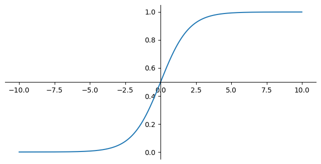
시그모이드 형태를 이용해서, 결과가 0.7이라면 악성일 확률이 70%라고 판단.
💻실습
import pandas as pd
wine_url = "https://raw.githubusercontent.com/PinkWink/ML_tutorial/master/dataset/wine.csv"

wine = pd.read_csv(wine_url, index_col=0)
wine.head()| fixed acidity | volatile acidity | citric acid | residual sugar | chlorides | free sulfur dioxide | total sulfur dioxide | density | pH | sulphates | alcohol | quality | color | |
|---|---|---|---|---|---|---|---|---|---|---|---|---|---|
| 0 | 7.4 | 0.70 | 0.00 | 1.9 | 0.076 | 11.0 | 34.0 | 0.9978 | 3.51 | 0.56 | 9.4 | 5 | 1 |
| 1 | 7.8 | 0.88 | 0.00 | 2.6 | 0.098 | 25.0 | 67.0 | 0.9968 | 3.20 | 0.68 | 9.8 | 5 | 1 |
| 2 | 7.8 | 0.76 | 0.04 | 2.3 | 0.092 | 15.0 | 54.0 | 0.9970 | 3.26 | 0.65 | 9.8 | 5 | 1 |
| 3 | 11.2 | 0.28 | 0.56 | 1.9 | 0.075 | 17.0 | 60.0 | 0.9980 | 3.16 | 0.58 | 9.8 | 6 | 1 |
| 4 | 7.4 | 0.70 | 0.00 | 1.9 | 0.076 | 11.0 | 34.0 | 0.9978 | 3.51 | 0.56 | 9.4 | 5 | 1 |
# 맛 등급 컬럼 생성
wine['taste'] = [1. if grade > 5 else 0. for grade in wine['quality']]
X = wine.drop(['taste','quality'], axis=1)
y = wine['taste']
# 데이터 분리
from sklearn.model_selection import train_test_split
X_train,X_test,y_train,y_test = train_test_split(X,y, test_size=0.2, random_state=13)💡로지스틱 회귀 간단 테스트
from sklearn.linear_model import LogisticRegression
from sklearn.metrics import accuracy_score

lr = LogisticRegression(solver='liblinear', random_state=13)  #solver=최적화 알고리즘을 무엇으로 잡을지 설정
lr.fit(X_train,y_train)

y_pred_tr = lr.predict(X_train)
y_pred_test = lr.predict(X_test)

print('Train Acc : ', accuracy_score(y_train,y_pred_tr))
print('Test Acc : ', accuracy_score(y_test,y_pred_test))
Train Acc : 0.7427361939580527
Test Acc : 0.7438461538461538로지스틱 회귀로 확인한 와인의 맛 분류 [0/1] 의 정확도는 74%정도
# 스케일러까지 적용해서 파이프라인 구축
from sklearn.pipeline import Pipeline
from sklearn.preprocessing import StandardScaler

estimators = [('scaler', StandardScaler()),
              ('clf' , LogisticRegression(solver='liblinear', random_state=13))]

pipe = Pipeline(estimators)
pipe.fit(X_train, y_train)pipe.fit(X_train, y_train)y_pred_tr = pipe.predict(X_train)
y_pred_test = pipe.predict(X_test)
print('Train Acc : ', accuracy_score(y_train,y_pred_tr))
print('Test Acc : ', accuracy_score(y_test,y_pred_test))Train Acc : 0.7444679622859341
Test Acc : 0.7469230769230769💡Decision Tree와의 비교
from sklearn.tree import DecisionTreeClassifier

wine_tree = DecisionTreeClassifier(max_depth=2, random_state=13)
wine_tree.fit(X_train, y_train)

models = {
    'logistic regression' : pipe,
    'decision tree' : wine_tree
}
from sklearn.metrics import roc_curve
plt.figure(figsize=(10,8))
plt.plot([0,1],[0,1], label='random_guess') #0,0과 1,1 잇는 기준선
for model_name, model in models.items():
pred = model.predict_proba(X_test)[:,1] #1일 확률
fpr, tpr, thresholds = roc_curve(y_test, pred)
plt.plot(fpr,tpr, label=model_name)
plt.grid()
plt.legend()
plt.show()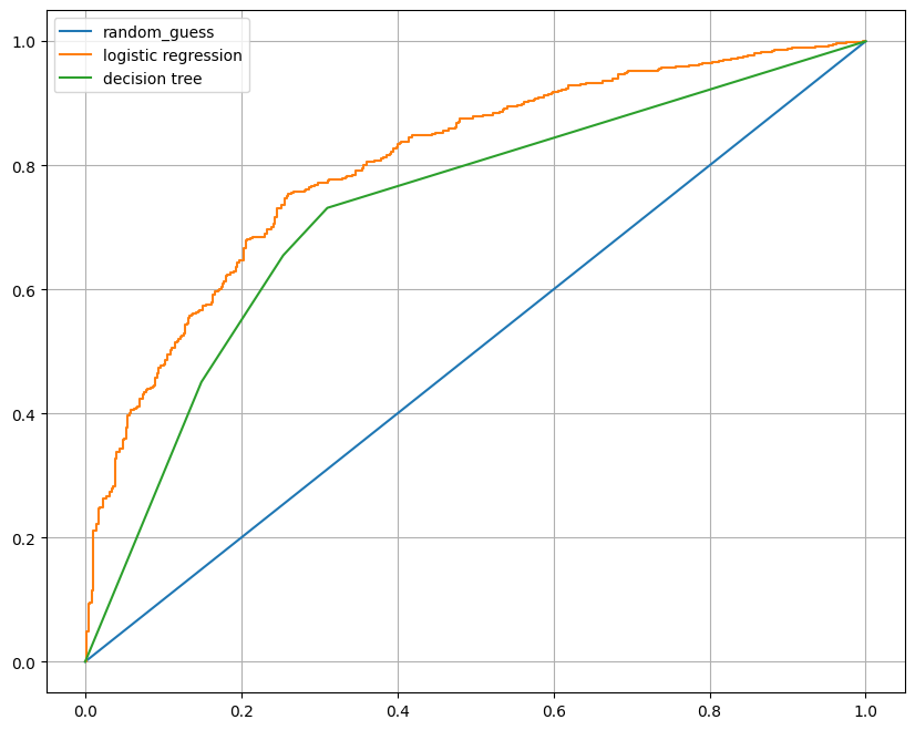
Logistic Regression 성능이 가장 좋음
📙PIMA 인디언 당뇨병 예측
50년대까지 PIMA인디언은 당뇨가 없었음 -> 20세기 말, 50년만에 인구의 50%가 당뇨에 걸림
PIMA_url = 'https://raw.githubusercontent.com/PinkWink/ML_tutorial/master/dataset/diabetes.csv'

PIMA = pd.read_csv(PIMA_url)
PIMA.head()| Pregnancies | Glucose | BloodPressure | SkinThickness | Insulin | BMI | DiabetesPedigreeFunction | Age | Outcome | |
|---|---|---|---|---|---|---|---|---|---|
| 0 | 6 | 148 | 72 | 35 | 0 | 33.6 | 0.627 | 50 | 1 |
| 1 | 1 | 85 | 66 | 29 | 0 | 26.6 | 0.351 | 31 | 0 |
| 2 | 8 | 183 | 64 | 0 | 0 | 23.3 | 0.672 | 32 | 1 |
| 3 | 1 | 89 | 66 | 23 | 94 | 28.1 | 0.167 | 21 | 0 |
| 4 | 0 | 137 | 40 | 35 | 168 | 43.1 | 2.288 | 33 | 1 |
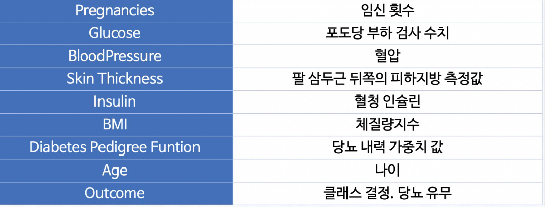
❔컬럼의 의미
PIMA.info()<class 'pandas.core.frame.DataFrame'>
RangeIndex: 768 entries, 0 to 767
Data columns (total 9 columns):
# Column Non-Null Count Dtype
--- ------ -------------- -----
0 Pregnancies 768 non-null int64
1 Glucose 768 non-null int64
2 BloodPressure 768 non-null int64
3 SkinThickness 768 non-null int64
4 Insulin 768 non-null int64
5 BMI 768 non-null float64
6 DiabetesPedigreeFunction 768 non-null float64
7 Age 768 non-null int64
8 Outcome 768 non-null int64
dtypes: float64(2), int64(7)
memory usage: 54.1 KB# float형으로 통일
PIMA = PIMA.astype('float')
PIMA.info()<class 'pandas.core.frame.DataFrame'>
RangeIndex: 768 entries, 0 to 767
Data columns (total 9 columns):
# Column Non-Null Count Dtype
--- ------ -------------- -----
0 Pregnancies 768 non-null float64
1 Glucose 768 non-null float64
2 BloodPressure 768 non-null float64
3 SkinThickness 768 non-null float64
4 Insulin 768 non-null float64
5 BMI 768 non-null float64
6 DiabetesPedigreeFunction 768 non-null float64
7 Age 768 non-null float64
8 Outcome 768 non-null float64
dtypes: float64(9)
memory usage: 54.1 KB#상관관계 확인
import seaborn as sns
plt.figure(figsize=(10,8))
sns.heatmap(PIMA.corr(), cmap='YlGnBu')
plt.show()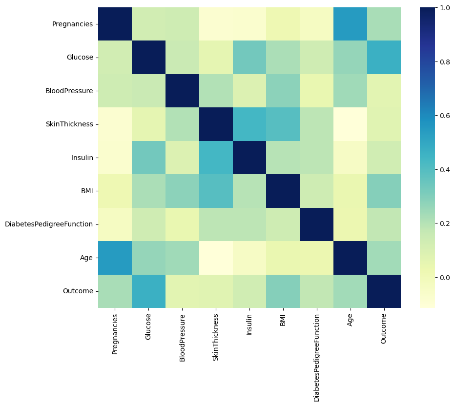
Outcomd과 다른 특성과의 관계를 보면 Pregnancies, Glucose, BMI, Age와 다소 관련이 있어보임
# EDA과정에서 '0'을 발견
(PIMA==0).astype(int).sum()
Pregnancies 111
Glucose 5
BloodPressure 35
SkinThickness 227
Insulin 374
BMI 11
DiabetesPedigreeFunction 0
Age 0
Outcome 500
dtype: int64# 0을 가지면 이상 데이터인 경우 처리 --> 평균 값으로 대체
zero_features = ['Glucose','BloodPressure','SkinThickness','BMI']
PIMA[zero_features] = PIMA[zero_features].replace(0, PIMA[zero_features].mean())
(PIMA==0).astype(int).sum()Pregnancies 111
Glucose 0
BloodPressure 0
SkinThickness 0
Insulin 374
BMI 0
DiabetesPedigreeFunction 0
Age 0
Outcome 500
dtype: int64# 데이터 나누기
X = PIMA.drop(['Outcome'],axis=1)
y = PIMA['Outcome']
X_train, X_test, y_train, y_test = train_test_split(X,y, test_size=0.2, random_state=13, stratify = y)# pipeline 만들기
estimators = [('scaler', StandardScaler()),
('clf' , LogisticRegression(solver='liblinear', random_state=13))]
pipe_lr = Pipeline(estimators)
pipe_lr.fit(X_train, y_train)
pred = pipe_lr.predict(X_test)print('Accuracy : ', accuracy_score(y_test,pred))Accuracy : 0.7727272727272727💡Outcome을 제외한 8개 특성을 가진 다변수 방정식 각 계수 값 확인
coeff = list(pipe_lr['clf'].coef_[0])
labels = list(X_train.columns)

coeff
[0.3542658884412649,
1.201424442503758,
-0.1584013553628671,
0.033946577129299535,
-0.1628647195398812,
0.620404521989511,
0.36669355795578734,
0.17195965447035097]💡중요 feature에 대해 그려보기
features = pd.DataFrame({'Features' : labels, 'importance':coeff})
features.sort_values(by=['importance'],ascending=True,inplace=True)
features['positive'] = features['importance'] > 0
features.set_index('Features', inplace=True)
features['importance'].plot(kind='barh',
                           figsize=(10,7),
                           color = features['positive'].map({True:'blue',False:'red'}))
plt.xlabel('importance')
plt.show()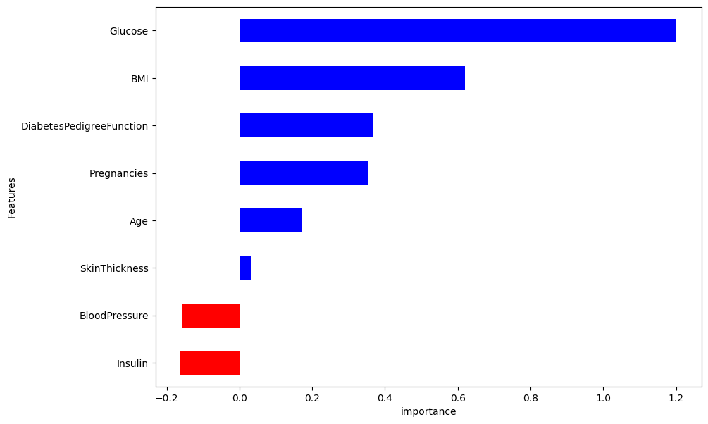
✔ 포도당, BMI등은 당뇨 영향에 미치는 정도가 높다.
✔ 혈압은 예측에 부정적 영향을 준다.
✔ 연령이 BMI보다 출력변수와 더 관련이 있었으나, 모델은 BMI와 Glucose에 더 의존함.

데이터분석 스터디노트🧐✍️