import pandas as pd
import numpy as np
import matplotlib.pyplot as plt
import seaborn as sns
data_url = 'https://raw.githubusercontent.com/PinkWink/ML_tutorial/master/dataset/ecommerce.csv'
data = pd.read_csv(data_url)
data.head()| Address | Avatar | Avg. Session Length | Time on App | Time on Website | Length of Membership | Yearly Amount Spent | ||
|---|---|---|---|---|---|---|---|---|
| 0 | mstephenson@fernandez.com | 835 Frank Tunnel\nWrightmouth, MI 82180-9605 | Violet | 34.497268 | 12.655651 | 39.577668 | 4.082621 | 587.951054 |
| 1 | hduke@hotmail.com | 4547 Archer Common\nDiazchester, CA 06566-8576 | DarkGreen | 31.926272 | 11.109461 | 37.268959 | 2.664034 | 392.204933 |
| 2 | pallen@yahoo.com | 24645 Valerie Unions Suite 582\nCobbborough, D... | Bisque | 33.000915 | 11.330278 | 37.110597 | 4.104543 | 487.547505 |
| 3 | riverarebecca@gmail.com | 1414 David Throughway\nPort Jason, OH 22070-1220 | SaddleBrown | 34.305557 | 13.717514 | 36.721283 | 3.120179 | 581.852344 |
| 4 | mstephens@davidson-herman.com | 14023 Rodriguez Passage\nPort Jacobville, PR 3... | MediumAquaMarine | 33.330673 | 12.795189 | 37.536653 | 4.446308 | 599.406092 |
- E-커머스 회사 고객 정보 데이터
- Avg.session Length : 한번 접속했을 때 평균 어느정도 시간을 사용하는지
- time on App : 폰 앱으로 접속했을 때 유지 시간(분)
- time on Website : 사이트로 접속했을 때 유지 시간 (분)
- Length on Membership :회원자격 유지 기간 (년)
# 필요없는 데이터 삭제
data.drop(['Email','Address','Avatar'],axis=1, inplace=True)
data.info()<class 'pandas.core.frame.DataFrame'>
RangeIndex: 500 entries, 0 to 499
Data columns (total 5 columns):
# Column Non-Null Count Dtype
--- ------ -------------- -----
0 Avg. Session Length 500 non-null float64
1 Time on App 500 non-null float64
2 Time on Website 500 non-null float64
3 Length of Membership 500 non-null float64
4 Yearly Amount Spent 500 non-null float64
dtypes: float64(5)
memory usage: 19.7 KBplt.figure(figsize=(12,6))
sns.boxplot(data=data.iloc[:,:-1]);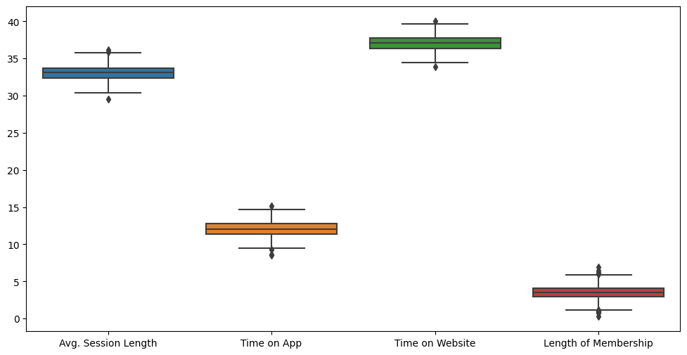
#Yearly만 따로 확인
plt.figure(figsize=(10,4))
sns.boxplot(data=data['Yearly Amount Spent']);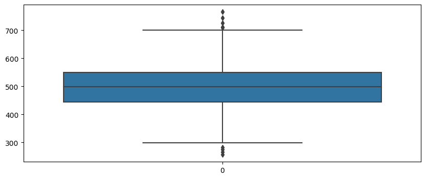
# pairplot으로 확인
plt.figure(figsize=(12,6))
sns.pairplot(data=data);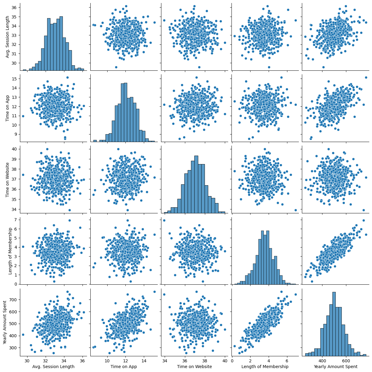
# lmplot으로 확인해보기
plt.figure(figsize=(12,6))
sns.lmplot(x='Length of Membership', y='Yearly Amount Spent', data = data);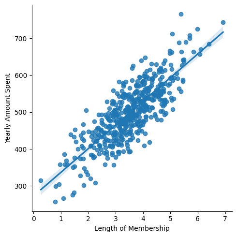
# 상관이 높은 멤버십 유지기간만 가지고 통계적 회귀

# statsmodels 패키지에 있는 ols 함수를 사용하면 간편하게 단순선형회귀 분석을 진행할 수 있다.
import statsmodels.api as sm

X = data['Length of Membership']
y = data['Yearly Amount Spent']
lm = sm.OLS(y,X).fit()
lm.summary()| Dep. Variable: | Yearly Amount Spent | R-squared (uncentered): | 0.970 |
|---|---|---|---|
| Model: | OLS | Adj. R-squared (uncentered): | 0.970 |
| Method: | Least Squares | F-statistic: | 1.617e+04 |
| Date: | Tue, 17 Jan 2023 | Prob (F-statistic): | 0.00 |
| Time: | 15:22:54 | Log-Likelihood: | -2945.2 |
| No. Observations: | 500 | AIC: | 5892. |
| Df Residuals: | 499 | BIC: | 5897. |
| Df Model: | 1 | ||
| Covariance Type: | nonrobust |
| coef | std err | t | P>|t| | [0.025 | 0.975] | |
|---|---|---|---|---|---|---|
| Length of Membership | 135.6117 | 1.067 | 127.145 | 0.000 | 133.516 | 137.707 |
| Omnibus: | 1.408 | Durbin-Watson: | 1.975 |
|---|---|---|---|
| Prob(Omnibus): | 0.494 | Jarque-Bera (JB): | 1.472 |
| Skew: | 0.125 | Prob(JB): | 0.479 |
| Kurtosis: | 2.909 | Cond. No. | 1.00 |
Notes:
[1] R² is computed without centering (uncentered) since the model does not contain a constant.
[2] Standard Errors assume that the covariance matrix of the errors is correctly specified.
분석 결과 해석
위 회귀분석 결과에서 나오는 주요 결과물들의 설명
Dep. Variable: Dependent variable, 종속변수를 의미한다.Model: 모델링 방법을 뜻하고, OLS는 Ordinary Least Squares의 약자이다.
▪ 참고로 OLS란, 최소제곱법, 또는 최소자승법, 최소제곱근사법, 이라고도 하며, 어떤 계의 해방정식을 근사적으로 구하는 방법으로서 근사적으로 구하려는 해와 실제 해의 오차의 제곱의 합이 최소가 되는 해를 구하는 방법이다.No. Observations: Number of observations, 관찰표본 수, 즉 총 표본 수를 뜻한다.Df Residuals: DF는 Degree of Freedom, 자유도를 뜻하는데, DF Residuals는 전체 표본 수에서 측정되는 변수들(종속변수 및 독립변수)의 개수를 빼서 구한다.Df Model: 독립변수의 개수.R squared: R의 제곱이라는 뜻이고 결정계수를 의미한다. 전체 데이터 중 해당 회귀모델이 설명할 수 있는 데이터의 비율, 회귀식의 설명력을 나타낸다. SSTr/SST이나 상관계수 R을 제곱해서 구할 수 있다.Adj. R-squared: 독립변수가 여러 개인 다중회귀분석에서 사용Prob. F-Statistic: 회귀 모형에 대한 통계적 유의미성 검정, 이 값이 0.05 이하라면 모집단에서도 의미가 있다고 볼 수 있음.F-statistics: F통계량, MSR/MSE로 구할 수 있다.Prob: F통계량에 해당하는 P-value를 의미.
결정계수; R squared 값 직접 구해서 비교해보기
- SSE = Sum of Squares for Errors (or Residuals) 잔차의 제곱합
- SSTr = Sum of Squares for Regression (or Treated) 회귀(예측값) 제곱합
- SST = Sum of Squares Total (SSE + SSTr)
- 결정계수 = SSTr / SST
# 회귀 모델 확인
pred = lm.predict(X)

sns.scatterplot(x=X, y=y)
plt.plot(X,pred,'r',ls='dashed',lw=3)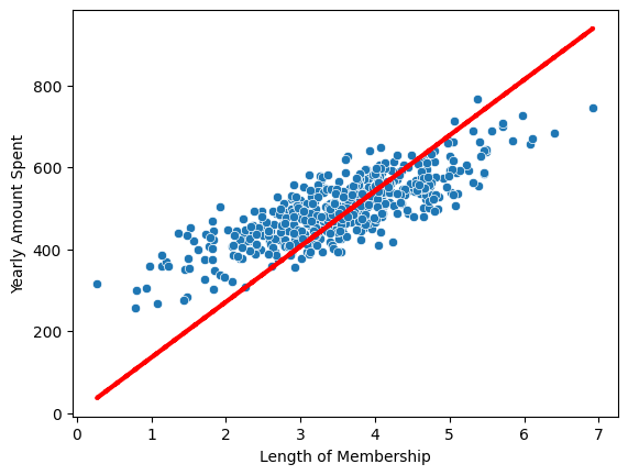
위의 값은 상수항이 없기 때문.
X에 열을 추가
X = np.c_[X, [1]*len(X)]
X[:5]
array([[4.08262063, 1. ],
[2.66403418, 1. ],
[4.1045432 , 1. ],
[3.12017878, 1. ],
[4.44630832, 1. ]])#다시 fit시키기
lm = sm.OLS(y,X).fit()
lm.summary()| Dep. Variable: | Yearly Amount Spent | R-squared: | 0.655 |
|---|---|---|---|
| Model: | OLS | Adj. R-squared: | 0.654 |
| Method: | Least Squares | F-statistic: | 943.9 |
| Date: | Tue, 17 Jan 2023 | Prob (F-statistic): | 4.81e-117 |
| Time: | 15:31:57 | Log-Likelihood: | -2629.9 |
| No. Observations: | 500 | AIC: | 5264. |
| Df Residuals: | 498 | BIC: | 5272. |
| Df Model: | 1 | ||
| Covariance Type: | nonrobust |
| coef | std err | t | P>|t| | [0.025 | 0.975] | |
|---|---|---|---|---|---|---|
| x1 | 64.2187 | 2.090 | 30.723 | 0.000 | 60.112 | 68.326 |
| const | 272.3998 | 7.675 | 35.492 | 0.000 | 257.320 | 287.479 |
| Omnibus: | 1.092 | Durbin-Watson: | 2.065 |
|---|---|---|---|
| Prob(Omnibus): | 0.579 | Jarque-Bera (JB): | 1.122 |
| Skew: | 0.037 | Prob(JB): | 0.571 |
| Kurtosis: | 2.780 | Cond. No. | 14.4 |
Notes:
[1] Standard Errors assume that the covariance matrix of the errors is correctly specified.
R-squared값과 AIC값이 낮아진 것을 알 수 있다.
pred = lm.predict(X)

sns.scatterplot(x=X[:,0],y=y)
plt.plot(X[:,0],pred,'r',ls='dashed',lw=3)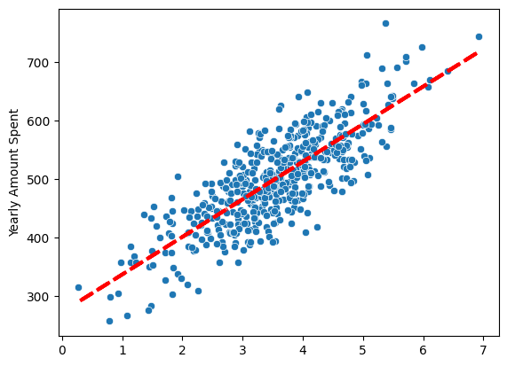
더 잘 반영된 위 모델 보다 상수항 반영되지 않은 첫번째 그래프 R-squared값이 더 높기 때문에 R-squared 자체를 무조건 신뢰해서는 안된다.
데이터 분리 후 평가
from sklearn.model_selection import train_test_split
X = data.drop('Yearly Amount Spent',axis=1)
y = data['Yearly Amount Spent']

X_train,X_test,y_train,y_test = train_test_split(X,y,test_size=0.2, random_state=13)
# 네개의 컬럼 모두를 변수로 보고 회귀
lm = sm.OLS(y_train,X_train).fit()
lm.summary()| Dep. Variable: | Yearly Amount Spent | R-squared (uncentered): | 0.998 |
|---|---|---|---|
| Model: | OLS | Adj. R-squared (uncentered): | 0.998 |
| Method: | Least Squares | F-statistic: | 4.884e+04 |
| Date: | Tue, 17 Jan 2023 | Prob (F-statistic): | 0.00 |
| Time: | 15:48:30 | Log-Likelihood: | -1816.5 |
| No. Observations: | 400 | AIC: | 3641. |
| Df Residuals: | 396 | BIC: | 3657. |
| Df Model: | 4 | ||
| Covariance Type: | nonrobust |
| coef | std err | t | P>|t| | [0.025 | 0.975] | |
|---|---|---|---|---|---|---|
| Avg. Session Length | 12.0166 | 0.832 | 14.440 | 0.000 | 10.381 | 13.653 |
| Time on App | 35.2145 | 1.129 | 31.197 | 0.000 | 32.995 | 37.434 |
| Time on Website | -14.4797 | 0.774 | -18.715 | 0.000 | -16.001 | -12.959 |
| Length of Membership | 60.7148 | 1.151 | 52.742 | 0.000 | 58.452 | 62.978 |
| Omnibus: | 0.449 | Durbin-Watson: | 2.036 |
|---|---|---|---|
| Prob(Omnibus): | 0.799 | Jarque-Bera (JB): | 0.571 |
| Skew: | -0.038 | Prob(JB): | 0.752 |
| Kurtosis: | 2.832 | Cond. No. | 54.7 |
Notes:
[1] R² is computed without centering (uncentered) since the model does not contain a constant.
[2] Standard Errors assume that the covariance matrix of the errors is correctly specified.
# 참 값, 예측 값
pred = lm.predict(X_test)

sns.scatterplot(x=y_test,y=pred)
plt.plot([min(y_test),max(y_test)], [min(y_test), max(y_test)],'r',ls='dashed',lw=3);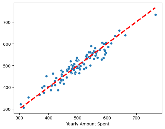

데이터분석 스터디노트🧐✍️