
1.데이터 읽어오기
- customer_master.csv 고객 데이터, 이름, 성별 등
- item_master.csv 취급하는 상품 데이터, 상품명, 가격 등
- transaction_1.csv 구매내역 데이터
3-1 transaction_2.csv 3과 연결된 구매내역 분할 데이터 - transaction_detail_1.csv 구매내역 상세 데이터
4-1 transaction_detail_2.csv 4와 연결된 분할 데이터
import pandas as pd
import warnings
warnings.filterwarnings('ignore')

customer_master = pd.read_csv('customer_master.csv')
customer_master.head()| customer_id | customer_name | registration_date | gender | age | birth | pref | ||
|---|---|---|---|---|---|---|---|---|
| 0 | IK152942 | 김서준 | 2019-01-01 0:25 | hirata_yuujirou@example.com | M | 29 | 1990-06-10 | 대전광역시 |
| 1 | TS808488 | 김예준 | 2019-01-01 1:13 | tamura_shiori@example.com | F | 33 | 1986-05-20 | 인천광역시 |
| 2 | AS834628 | 김도윤 | 2019-01-01 2:00 | hisano_yuki@example.com | F | 63 | 1956-01-02 | 광주광역시 |
| 3 | AS345469 | 김시우 | 2019-01-01 4:48 | tsuruoka_kaoru@example.com | M | 74 | 1945-03-25 | 인천광역시 |
| 4 | GD892565 | 김주원 | 2019-01-01 4:54 | oouchi_takashi@example.com | M | 54 | 1965-08-05 | 울산광역시 |
item_master = pd.read_csv('item_master.csv')
item_master.head()| item_id | item_name | item_price | |
|---|---|---|---|
| 0 | S001 | PC-A | 50000 |
| 1 | S002 | PC-B | 85000 |
| 2 | S003 | PC-C | 120000 |
| 3 | S004 | PC-D | 180000 |
| 4 | S005 | PC-E | 210000 |
transaction_1 = pd.read_csv('transaction_1.csv')
transaction_1.head()| transaction_id | price | payment_date | customer_id | |
|---|---|---|---|---|
| 0 | T0000000113 | 210000 | 2019-02-01 01:36:57 | PL563502 |
| 1 | T0000000114 | 50000 | 2019-02-01 01:37:23 | HD678019 |
| 2 | T0000000115 | 120000 | 2019-02-01 02:34:19 | HD298120 |
| 3 | T0000000116 | 210000 | 2019-02-01 02:47:23 | IK452215 |
| 4 | T0000000117 | 170000 | 2019-02-01 04:33:46 | PL542865 |
transaction_detail_1 = pd.read_csv('transaction_detail_1.csv')
transaction_detail_1.head()| detail_id | transaction_id | item_id | quantity | |
|---|---|---|---|---|
| 0 | 0 | T0000000113 | S005 | 1 |
| 1 | 1 | T0000000114 | S001 | 1 |
| 2 | 2 | T0000000115 | S003 | 1 |
| 3 | 3 | T0000000116 | S005 | 1 |
| 4 | 4 | T0000000117 | S002 | 2 |
우선 가지고 있는 데이터 전체를 파악하는 것이 중요하다. 또, 분석 목적에 따라 다르겠으나 되도록이면 상세하게 나와있는 쪽에 맞추어 가공하는 것이 좋다.
transaction_detail을 기준으로 생각할 경우, 크게 2가지 데이터 가공이 필요한데 첫번째로 3,3-1/4,4-1로 분할된 데이터를 세로로 결합(유니언)하는 것. 두번째로는 transaction_detail을 기준으로 transaction, customer_master, item_master를 가로로 결합(조인)하는 것이다.
2.데이터 결합 (유니언)
transaction_2 = pd.read_csv('transaction_2.csv')
transaction = pd.concat([transaction_1,transaction_2],ignore_index=True)
transaction.head()| transaction_id | price | payment_date | customer_id | |
|---|---|---|---|---|
| 0 | T0000000113 | 210000 | 2019-02-01 01:36:57 | PL563502 |
| 1 | T0000000114 | 50000 | 2019-02-01 01:37:23 | HD678019 |
| 2 | T0000000115 | 120000 | 2019-02-01 02:34:19 | HD298120 |
| 3 | T0000000116 | 210000 | 2019-02-01 02:47:23 | IK452215 |
| 4 | T0000000117 | 170000 | 2019-02-01 04:33:46 | PL542865 |
# 데이터 수 확인
print(len(transaction_1))
print(len(transaction_2))
print(len(transaction))
5000
1786
6786transaction_detail_2 = pd.read_csv('transaction_detail_2.csv')
transaction_detail=pd.concat([transaction_detail_1,transaction_detail_2], ignore_index=True)
transaction_detail.head()| detail_id | transaction_id | item_id | quantity | |
|---|---|---|---|---|
| 0 | 0 | T0000000113 | S005 | 1 |
| 1 | 1 | T0000000114 | S001 | 1 |
| 2 | 2 | T0000000115 | S003 | 1 |
| 3 | 3 | T0000000116 | S005 | 1 |
| 4 | 4 | T0000000117 | S002 | 2 |
3. 매출데이터 결합 (조인)
데이터를 조인할 때는 기준이 되는 데이터를 정확하게 결정하고, 어떤 컬럼을 키로 조인할지 생각해야함.
가장 상세한 데이터인 transaction_detail을 기준으로 한다면, 우선 조인할때 1.부족하거나 추가하고 싶은 컬럼이 무엇인지와 2. 공통되는 컬럼이 무엇인지 생각한다.
join_data = pd.merge(transaction_detail, transaction[['transaction_id','payment_date','customer_id']],
                     on='transaction_id',how='left')
join_data.head()| detail_id | transaction_id | item_id | quantity | payment_date | customer_id | |
|---|---|---|---|---|---|---|
| 0 | 0 | T0000000113 | S005 | 1 | 2019-02-01 01:36:57 | PL563502 |
| 1 | 1 | T0000000114 | S001 | 1 | 2019-02-01 01:37:23 | HD678019 |
| 2 | 2 | T0000000115 | S003 | 1 | 2019-02-01 02:34:19 | HD298120 |
| 3 | 3 | T0000000116 | S005 | 1 | 2019-02-01 02:47:23 | IK452215 |
| 4 | 4 | T0000000117 | S002 | 2 | 2019-02-01 04:33:46 | PL542865 |
print(len(transaction_detail))
print(len(transaction))
print(len(join_data))
7144
6786
7144join은 가로로 데이터가 늘어나기 때문에 데이터 갯수는 동일하다. 단, 조인할 데이터의 조인키 (여기서는 customer_id)에 중복데이터가 있을 경우 데이터 개수가 늘어날 수 있기 때문에 주의!
4. 마스터 데이터를 결합(조인)하기
이번에는 customer_master와 item_master에 포함된 데이터로, 공통 컬럼은 각 customer_id, item_id로 연결 가능하다.
join_data = pd.merge(join_data, customer_master, on='customer_id',how='left')
join_data = pd.merge(join_data, item_master, on='item_id', how='left')
join_data.head()| detail_id | transaction_id | item_id | quantity | payment_date | customer_id | customer_name | registration_date | gender | age | birth | pref | item_name | item_price | ||
|---|---|---|---|---|---|---|---|---|---|---|---|---|---|---|---|
| 0 | 0 | T0000000113 | S005 | 1 | 2019-02-01 01:36:57 | PL563502 | 김태경 | 2019-01-07 14:34 | imoto_yoshimasa@example.com | M | 30 | 1989-07-15 | 대전광역시 | PC-E | 210000 |
| 1 | 1 | T0000000114 | S001 | 1 | 2019-02-01 01:37:23 | HD678019 | 김영웅 | 2019-01-27 18:00 | mifune_rokurou@example.com | M | 73 | 1945-11-29 | 서울특별시 | PC-A | 50000 |
| 2 | 2 | T0000000115 | S003 | 1 | 2019-02-01 02:34:19 | HD298120 | 김강현 | 2019-01-11 8:16 | yamane_kogan@example.com | M | 42 | 1977-05-17 | 광주광역시 | PC-C | 120000 |
| 3 | 3 | T0000000116 | S005 | 1 | 2019-02-01 02:47:23 | IK452215 | 김주한 | 2019-01-10 5:07 | ikeda_natsumi@example.com | F | 47 | 1972-03-17 | 인천광역시 | PC-E | 210000 |
| 4 | 4 | T0000000117 | S002 | 2 | 2019-02-01 04:33:46 | PL542865 | 김영빈 | 2019-01-25 6:46 | kurita_kenichi@example.com | M | 74 | 1944-12-17 | 광주광역시 | PC-B | 85000 |
5. 필요한 컬럼 만들기
결합으로 인해 사라진 매출(price)데이터를 만들어보기. 매출은 quantity와 item_price의 곱을 계산하여 추가할 수 있다.
join_data['price'] = join_data['quantity'] * join_data['item_price']
join_data[['quantity','item_price','price']].head()| quantity | item_price | price | |
|---|---|---|---|
| 0 | 1 | 210000 | 210000 |
| 1 | 1 | 50000 | 50000 |
| 2 | 1 | 120000 | 120000 |
| 3 | 1 | 210000 | 210000 |
| 4 | 2 | 85000 | 170000 |
6. 데이터 검산
데이터 가공 단계에서 집계 실수 등으로 수치상 에러가 생기는 경우를 막기 위해 검산 가능한 경우 꼭 확인해보기.
join_data['price'].sum() == transaction['price'].sum()True7.데이터 분석 (각종 통계랑 파악)
데이터 분석 시 크게 두가지 숫자를 파악해야한다. 첫번째로는 결손치의 개수, 두번째는 전체를 파악할 수 있는 숫자감이다.
결손치의 경우 항상 포함될 가능성이 있으므로, 숫자를 파악해서 제거하거나 보간해야된다.
또 분석에서는 상품별, 고객별 등 다양하게 집계를 하는데, 가령 이번달 A의 매출이 10만원이라 한다면 전체매출 단위가 100억인지, 100만원인지에 따라서도 의미가 크게 다르기 때문에 전체적인 숫자감을 파악하는게 중요하다.
join_data.isnull().sum()detail_id 0
transaction_id 0
item_id 0
quantity 0
payment_date 0
customer_id 0
customer_name 0
registration_date 0
email 0
gender 0
age 0
birth 0
pref 0
item_name 0
item_price 0
price 0
dtype: int64join_data.describe()| detail_id | quantity | age | item_price | price | |
|---|---|---|---|---|---|
| count | 7144.000000 | 7144.000000 | 7144.000000 | 7144.000000 | 7144.000000 |
| mean | 3571.500000 | 1.199888 | 50.265677 | 121698.628219 | 135937.150056 |
| std | 2062.439494 | 0.513647 | 17.190314 | 64571.311830 | 68511.453297 |
| min | 0.000000 | 1.000000 | 20.000000 | 50000.000000 | 50000.000000 |
| 25% | 1785.750000 | 1.000000 | 36.000000 | 50000.000000 | 85000.000000 |
| 50% | 3571.500000 | 1.000000 | 50.000000 | 102500.000000 | 120000.000000 |
| 75% | 5357.250000 | 1.000000 | 65.000000 | 187500.000000 | 210000.000000 |
| max | 7143.000000 | 4.000000 | 80.000000 | 210000.000000 | 420000.000000 |
describe를 활용해서 전반적으로 데이터 분포를 확인하자.
추가로 확인할 수있는 기간 데이터도 확인해보자.
print(join_data['payment_date'].min())
print(join_data['payment_date'].max())
2019-02-01 01:36:57
2019-07-31 23:41:38전체 데이터의 기간은 2019-02-01~2019-07-31 사이인 것을 알 수 있다.
8.월별 데이터 집계하기
시계열 상황을 확인해서 매출이 어떠한 흐름으로 늘어나거나 줄어드는지 파악해보기.
join_data.dtypesdetail_id int64
transaction_id object
item_id object
quantity int64
payment_date object
customer_id object
customer_name object
registration_date object
email object
gender object
age int64
birth object
pref object
item_name object
item_price int64
price int64
dtype: object# date를 object에서 datetime으로 변환
join_data['payment_date'] = pd.to_datetime(join_data['payment_date'])
join_data['payment_month'] = join_data['payment_date'].dt.strftime('%Y%m')
join_data[['payment_date','payment_month']].head()| payment_date | payment_month | |
|---|---|---|
| 0 | 2019-02-01 01:36:57 | 201902 |
| 1 | 2019-02-01 01:37:23 | 201902 |
| 2 | 2019-02-01 02:34:19 | 201902 |
| 3 | 2019-02-01 02:47:23 | 201902 |
| 4 | 2019-02-01 04:33:46 | 201902 |
datetime형으로 변환한 후에 새로운 컬럼 (payment_month)를 연월단위로 작성했다.
판다스의 datetime의 dt를 사용하면 년/월 추출이 가능하다.
# 집계해보기
join_data.groupby('payment_month').sum()| detail_id | quantity | age | item_price | price | |
|---|---|---|---|---|---|
| payment_month | |||||
| 201902 | 676866 | 1403 | 59279 | 142805000 | 160185000 |
| 201903 | 2071474 | 1427 | 58996 | 142980000 | 160370000 |
| 201904 | 3476816 | 1421 | 59246 | 143670000 | 160510000 |
| 201905 | 4812795 | 1390 | 58195 | 139655000 | 155420000 |
| 201906 | 6369999 | 1446 | 61070 | 147090000 | 164030000 |
| 201907 | 8106846 | 1485 | 62312 | 153215000 | 170620000 |
# 위의 집계 내역에서 price만 보고싶다면? 월별 '매출' 집계 확인 시 ['price']컬럼 추가
join_data.groupby('payment_month').sum()['price']
payment_month
201902 160185000
201903 160370000
201904 160510000
201905 155420000
201906 164030000
201907 170620000
Name: price, dtype: int645월에 매출이 약간 내려갔지만 6,7월에 회복을 했으며, 반년 간 가장 매출이 높은 달은 7월이다. 한달에 대략 1억6천만원 정도 매출이 나오고 있으며, 연간 20억 정도 매출이 기대된다.
이번엔 월별 및 상품별로 집계해서 확인해보자.
9. 월별, 상품별로 데이터를 집계해보자
join_data.groupby(['payment_month','item_name']).sum()[['price','quantity']]| price | quantity | ||
|---|---|---|---|
| payment_month | item_name | ||
| 201902 | PC-A | 24150000 | 483 |
| PC-B | 25245000 | 297 | |
| PC-C | 19800000 | 165 | |
| PC-D | 31140000 | 173 | |
| PC-E | 59850000 | 285 | |
| 201903 | PC-A | 26000000 | 520 |
| PC-B | 25500000 | 300 | |
| PC-C | 19080000 | 159 | |
| PC-D | 25740000 | 143 | |
| PC-E | 64050000 | 305 | |
| 201904 | PC-A | 25900000 | 518 |
| PC-B | 23460000 | 276 | |
| PC-C | 21960000 | 183 | |
| PC-D | 24300000 | 135 | |
| PC-E | 64890000 | 309 | |
| 201905 | PC-A | 24850000 | 497 |
| PC-B | 25330000 | 298 | |
| PC-C | 20520000 | 171 | |
| PC-D | 25920000 | 144 | |
| PC-E | 58800000 | 280 | |
| 201906 | PC-A | 26000000 | 520 |
| PC-B | 23970000 | 282 | |
| PC-C | 21840000 | 182 | |
| PC-D | 28800000 | 160 | |
| PC-E | 63420000 | 302 | |
| 201907 | PC-A | 25250000 | 505 |
| PC-B | 28220000 | 332 | |
| PC-C | 19440000 | 162 | |
| PC-D | 26100000 | 145 | |
| PC-E | 71610000 | 341 |
좀더 직관적 확인을 위해 피벗 테이블로 집계해보기
pd.pivot_table(join_data, index='item_name',columns='payment_month',values=['price','quantity'],aggfunc='sum')| price | quantity | |||||||||||
|---|---|---|---|---|---|---|---|---|---|---|---|---|
| payment_month | 201902 | 201903 | 201904 | 201905 | 201906 | 201907 | 201902 | 201903 | 201904 | 201905 | 201906 | 201907 |
| item_name | ||||||||||||
| PC-A | 24150000 | 26000000 | 25900000 | 24850000 | 26000000 | 25250000 | 483 | 520 | 518 | 497 | 520 | 505 |
| PC-B | 25245000 | 25500000 | 23460000 | 25330000 | 23970000 | 28220000 | 297 | 300 | 276 | 298 | 282 | 332 |
| PC-C | 19800000 | 19080000 | 21960000 | 20520000 | 21840000 | 19440000 | 165 | 159 | 183 | 171 | 182 | 162 |
| PC-D | 31140000 | 25740000 | 24300000 | 25920000 | 28800000 | 26100000 | 173 | 143 | 135 | 144 | 160 | 145 |
| PC-E | 59850000 | 64050000 | 64890000 | 58800000 | 63420000 | 71610000 | 285 | 305 | 309 | 280 | 302 | 341 |
10. 시각화해서 확인
graph_data = pd.pivot_table(join_data,index='payment_month',columns='item_name',values='price',aggfunc='sum')
graph_data.head()| item_name | PC-A | PC-B | PC-C | PC-D | PC-E |
|---|---|---|---|---|---|
| payment_month | |||||
| 201902 | 24150000 | 25245000 | 19800000 | 31140000 | 59850000 |
| 201903 | 26000000 | 25500000 | 19080000 | 25740000 | 64050000 |
| 201904 | 25900000 | 23460000 | 21960000 | 24300000 | 64890000 |
| 201905 | 24850000 | 25330000 | 20520000 | 25920000 | 58800000 |
| 201906 | 26000000 | 23970000 | 21840000 | 28800000 | 63420000 |
import matplotlib.pyplot as plt
%matplotlib inline
plt.plot(list(graph_data.index),graph_data['PC-A'],label='PC-A')
plt.plot(list(graph_data.index),graph_data['PC-B'],label='PC-B')
plt.plot(list(graph_data.index),graph_data['PC-C'],label='PC-C')
plt.plot(list(graph_data.index),graph_data['PC-D'],label='PC-D')
plt.plot(list(graph_data.index),graph_data['PC-E'],label='PC-E')
plt.legend() # 각 라벨 범례표시<matplotlib.legend.Legend at 0x20ece560fd0>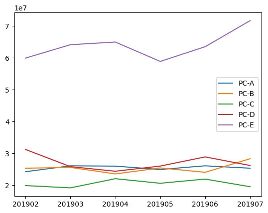
매출 추이 파악 및 PC-E가 매출을 견인하는 기종임을 확인할 수 있다.