파이토치(pytorch)

Define by run

• 연산이 이루어지는 시점에서 동적으로 그래프를 만들어 연산 수향
• 낮은 단위의 연산들로 구성할 수 있게 되고 디버깅 및 구조 설계의 세분화

auto grad

• 자동 미분
  : 연산 정보를 기억했다가 자동으로 미분 → requires- grad = true

https://colab.research.google.com/github/PyTorchKorea/tutorials-kr/blob/master/docs/_downloads/af0caf6d7af0dda755f4c9d7af9ccc2c/quickstart_tutorial.ipynb#scrollTo=D2mmlsfGwY3z

dataloader

• Dataset 을 DataLoader 의 인자로 전달합니다.
• 이는 데이터셋을 순회 가능한 객체(iterable)로 감싸고, 자동화된 배치(batch), 샘플링(sampling), 섞기(shuffle) 및 다중 프로세스로 데이터 불러오기(multiprocess data loading)를 지원

• linear : dense 역할 (특성 수)
• 4차원에서 2차원 변경을 위해 self.flatten = nn.Flatten()

X, y = X.to(device), y.to(device)

• gpu로 옮김

optimizer.zero_grad() : 반복을 위해 초기화

correct += (pred.argmax(1) == y).type(torch.float).sum().item()

• 정답과 비교

  tensor

  y3 = torch.rand_like(y1)
• 똑같은형상으로 랜덤하게 채움

torch.matmul(tensor, tensor.T, out=y3)

• y3의 결과를 저장

agg = tensor.sum()
agg_item = agg.item()
print(agg_item, type(agg_item))

• 바꿔치기(in-place) 연산 연산 결과를 피연산자(operand)에 저장하는 연산을 바꿔치기 연산이라고 부르며, 접미사를 갖습니다. 예를 들어: x.copy(y) 나 x.t_() 는 x 를 변경합니다.

• 기록이 즉시 삭제되어 계산에 문제가 될 수 있다.

  data_tutorial. (set, loader)

• DataLoader 는 Dataset 을 샘플에 쉽게 접근할 수 있도록 순회 가능한 객체(iterable)로 감쌉니다.

사용자 정의 Dataset 클래스는 반드시 3개 함수를 구현해야 합니다: init, len, and getitem. 아래 구현을 살펴보면 FashionMNIST 이미지들은 img_dir 디렉토리에 저장되고, 정답은 annotations_file csv 파일에 별도로 저장됩니다.

• 특정 이미지르 뽑아라

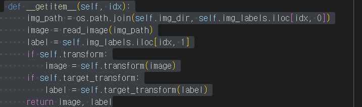
getitem

• getitem 함수는 주어진 인덱스 idx 에 해당하는 샘플을 데이터셋에서 불러오고 반환
• 인덱스를 기반으로, 디스크에서 이미지의 위치를 식별하고, read_image 를 사용하여 이미지를 텐서로 변환
• self.img_labels 의 csv 데이터로부터 해당하는 정답(label)을 가져오고, (해당하는 경우) 변형(transform) 함수들을 호출 뒤 텐서 이미지와 라벨을 Python 사전(dict)형으로 반환

ToTensor

• ToTensor 는 PIL Image나 NumPy ndarray 를 FloatTensor 로 변환
• 이미지의 픽셀의 크기(intensity) 값을 [0., 1.] 범위로 비례하여 조정(scale)합니다.

Lambda

• Lambda 변형은 사용자 정의 람다(lambda) 함수를 적용
• 여기에서는 정수를 원-핫으로 부호화된 텐서로 바꾸는 함수를 정의
• 이 함수는 먼저 (데이터셋 정답의 개수인) 크기 10짜리 영 텐서(zero tensor)를 만들고, scatter_ 를 호출
• 주어진 정답 y 에 해당하는 인덱스에 value=1 을 할당합니다.

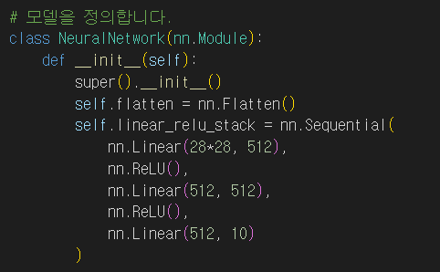
신경망모델 구성하기

nn.Flatten
nn.Flatten 계층을 초기화하여 각 28x28의 2D 이미지를 784 픽셀 값을 갖는 연속된 배열로 변환합니다. (dim=0의 미니배치 차원은 유지됩니다.)

nn.ReLU
비선형 활성화(activation)는 모델의 입력과 출력 사이에 복잡한 관계(mapping)를 만듭니다. 비선형 활성화는 선형 변환 후에 적용되어 비선형성(nonlinearity) 을 도입하고, 신경망이 다양한 현상을 학습할 수 있도록 돕습니다. - 음수는 전부 0

z = torch.matmul(x, w)+b
print(z.requires_grad)

with torch.no_grad():
z = torch.matmul(x, w)+b
requires_grad=True\ 인 모든 텐서들은 연산 기록을 추적

backward호출
각 .grad_fn 으로부터 변화도를 계산하고,
각 텐서의 .grad 속성에 계산 결과를 쌓고(accumulate),
연쇄 법칙을 사용하여, 모든 잎(leaf) 텐서들까지 전파(propagate)합니다.

모델 저장 불러오기

model = models.vgg16(weights='IMAGENET1K_V1')

torch.save(model.state_dict(), 'model_weights.pth')
모델 전체 저장

torch.manual_seed(1729)
r3 = torch.rand(2, 2)
print('\nr1과 일치:')
print(r3) # 동일한 시드값으로 인해 r1 값이 반복되어 행렬값으로 나옵니다.

 x = x.view(-1, self.num_flat_features(x))
 - view: reshape 역할 
 
 
 
 

clone

forward() 메소드에 여러 갈래의 계산 경로가 있고 원본 tensor와 그것의 복제본 모두 가 모델의 출력에 기여를 한다면, 두 tensor에 대한 autograd를 설정하는 모델 학습을 활성화 합니다. 만약 여러분의 source tensor가 autograd를 사용할 수 있다면 (일반적으로 학습 가중치의 집합이거나, 가중치를 포함하는 계산에서 파생된 경우), 여러분이 원하는 결과를 얻을 수 있습니다.

반면에 원본 tensor나 그것의 복제본 모두 가 변화도를 추적할 필요가 없다면, source tensor의 autograd가 꺼져있다면 clone을 사용할 수 있습니다.

a = torch.rand(2, 2, requires_grad=True) # autograd를 켭니다.
print(a)

b = a.clone()
print(b)

c = a.detach().clone()
print(c)

print(a)

a 를 requires_grad=True 옵션을 킨 상태로 생성합니다. 아직 이 선택적 인자를 다루지 않았지만, autograd 단원 동안만 다룰 것입니다.
a 를 출력할 때, requires_grad=True 속성을 가지고 있다고 알려줍니다 - 이 뜻은 autograd와 계산 히스토리 추적 기능을 켠다는 것입니다.
a 를 복제하고 그것을 b 라고 라벨을 붙입니다. b 를 출력할 때, 그것의 계산 히스토리가 추적되고 있다는 것을 확인할 수 있습니다 - a 의 autograd 설정에 내장되어 있는 기능이며, 이 설정은 계산 히스토리에 추가합니다.
a 를 c 에 복제를 하지만 detach() 를 먼저 호출을 합니다.
c 를 출력합니다. 계산 히스토리가 없다는 것을 확인할 수 있고, requires_grad=True 옵션이 없다는 것 또한 확인할 수 있습니다

out.backward()
print(a.grad)
plt.plot(a.detach(), a.grad.detach())

두번 미분 시 :
out.backward(retain = true)
print(a.grad)
plt.plot(a.detach(), a.grad.detach())

device = torch.device('cpu')
run_on_gpu = False
if torch.cuda.is_available():
device = torch.device('cuda')
run_on_gpu = True

x = torch.randn(2, 3, requires_grad=True)
y = torch.rand(2, 3, requires_grad=True)
z = torch.ones(2, 3, requires_grad=True)

with torch.autograd.profiler.profile(usecuda=run_on_gpu) as prf:
for in range(1000):
z = (z / x) * y

print(prf.key_averages().table(sort_by='self_cpu_time_total'))

• profile 성능 분석
  (perf)