머신 러닝 - Clustering

이상해씨·2021년 12월 5일

머신 러닝

목록 보기

27/27

◾Clustering

비지도 학습 : 정답 라벨있는 지도 학습과 달리 정답 라벨이 없는 데이터를 비슷한 특징끼리 군집화하여 새로운 데이터에 대한 결과를 예측하는 방법, 라벨이 없은 데이터로부터 패턴이나 형태를 찾아야하기 때문에 난이도가 있다.
- 군집(Clustering) : 비슷한 샘플을 모음
- 이상치 탐지(Outlier Detection) : 정상 데이터가 어떻게 보이는지 학습하여 비정상 샘플을 감지
- 밀도 추정 : 데이터셋의 확률 밀도 함수(Probability Density Function, PDF)를 추정, 이상치 탐지 등에 사용
K-Means : 군집화에서 가장 일반적인 알고리즘
- 군집 중심(centroid)이라는 임의의 지점을 선택해서 해당 중심에 가장 가까운 포인트들을 선택하는 군집화
- 거리 기반 알고리즘으로 속성의 개수가 매우 많을 경우 군집화의 정확도가 떨어진다.
- 초기 중심점 설정 -> 각 데이터는 가장 가까운 중심점에 소속 -> 중심점에 할당된 평균값으로 중심점 이동 -> 각 데이터 중심정 재할당 -> 중심점의 변경이 없으면 종료
  입력 : 훈련 집합 $\mathbb{X} = {x_1, x_2, ..., x_n}$ 군집의 개수 k
  출력 : 군집 집합 $C = {c_1, c_2, ..., c_k}$
  1. k개의 군집 중심 $Z = {z_1, z_2, ..., z_k}$ 를 초기화한다.
  2. while(True)
  3. for(i = 1 to n)
  4. $x_i$ 를 가장 가까운 군집 중심에 배정
  5. if (라인 3~4에서 이루어진 배정이 이전 루프에서의 배정과 같으면) break
  6. for(j = 1 to k)
  7. $z_j$ 에 배정된 샘플의 평균으로 $z_j$ 를 대치한다.
  8. for(j = 1 to k)
  9. $z_j$ 에 배정된 샘플을 $c_j$ 에 대입한다.

- IRIS 데이터 실습

import matplotlib.pyplot as plt
import numpy as np
import pandas as pd
import set_matplotlib_korean

from sklearn.preprocessing import scale
from sklearn.datasets import load_iris
from sklearn.cluster import KMeans

편의상 2개의 특성만 사용

iris = load_iris()

# 단위 생략후 넣기
cols = [each[:-5] for each in iris.feature_names]

iris_df = pd.DataFrame(data=iris.data, columns=cols)
feature = iris_df[['petal length', 'petal width']]
feature.head(2)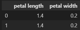

군집화 실습
- n_clusters : 군집화할 개수, 군집 중심정 개수
- init : 초기 군집 중심점의 좌표를 설정하는 방식 결정
- max_iter : 최대 반복 횟수, 모든 데이터의 중심점 이동이 없으면 종료

# 3개의 그룹으로 나눈다.
model = KMeans(n_clusters=3)
model.fit(feature)

KMeans의 결과 라벨은 지도학습의 라벨과는 다르다!!!

model.labels_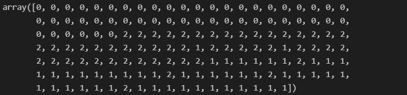

군집 중심값 확인

model.cluster_centers_

재정리

predict = pd.DataFrame(model.predict(feature), columns=['cluster'])
feature = pd.concat([feature, predict], axis=1)
feature.head()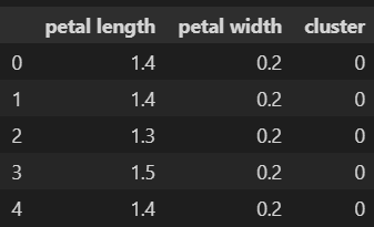

결과 확인

centers = pd.DataFrame(model.cluster_centers_,
                       columns=['petal length', 'petal width'])
center_x = centers['petal length']
center_y = centers['petal width']

plt.figure(figsize=(12, 8))
plt.scatter(feature['petal length'], feature['petal width'],
            c=feature['cluster'], alpha=0.5)
plt.scatter(center_x, center_y, s= 50, marker='D', c='r')
plt.show()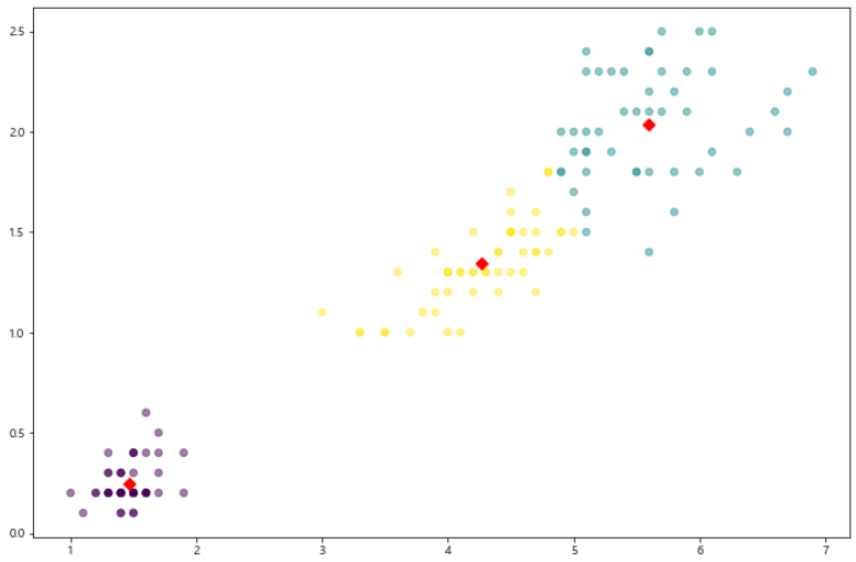

- make_blobs

make_blobs : 군집화 연습을 위한 데이터 생성기

from sklearn.datasets import make_blobs

X, y = make_blobs(n_samples=200, n_features=2, centers=3,
                  cluster_std=0.8, random_state=0)
print(X.shape, y.shape)

unique, counts = np.unique(y, return_counts=True)
print(unique, counts)

데이터 정리

cluster_df = pd.DataFrame(data=X, columns=['ftr1', 'ftr2'])
cluster_df['target'] = y
cluster_df.head()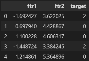

군집화

kmenas = KMeans(n_clusters=3, init='k-means++', max_iter=200, random_state=0)
cluster_labels = kmenas.fit_predict(X)
cluster_df['kmeans_label'] = cluster_labels

결과 도식화

centers = kmenas.cluster_centers_
unique_labels = np.unique(cluster_labels)
markers = ['o', 's', '^', 'P', 'D', 'H', 'x']

for label in unique_labels:
    label_cluster = cluster_df[cluster_df['kmeans_label'] == label]
    center_x_y = centers[label]
    plt.scatter(x=label_cluster['ftr1'], y=label_cluster['ftr2'], edgecolor='k', marker=markers[label])

    plt.scatter(x=center_x_y[0], y=center_x_y[1], s=200, color='white', alpha=0.9, edgecolor='k', marker=markers[label])

    plt.scatter(x=center_x_y[0], y=center_x_y[1], s=70, color='k', alpha=0.9, edgecolor='k', marker='$%d$' % label)

plt.show()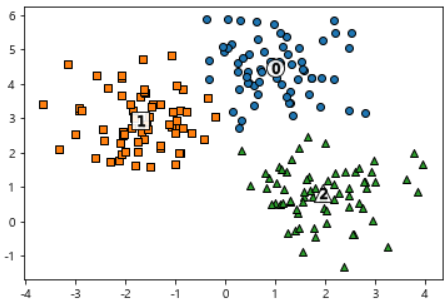

결과 확인

print(cluster_df.groupby('target')['kmeans_label'].value_counts())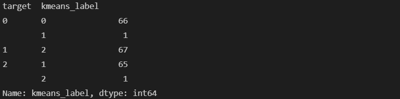

- 군집 평가

군집 결과의 평가
- 분류기는 평가 기준(정답)을 가지고 있지만, 군집은 그렇지 않다.
- 군집 결과를 평가하기 위해 실루엣 분석을 많이 활용한다.
실루엣 분석
- 실루엣 분석은 각 군집 간의 거리가 얼마나 효율적으로 분리되어 있느지 나타낸다.
- 다른 군집과는 거리가 떨어져있고, 동일 군집간의 데이터는서로 가깝게 잘 뭉쳐 있는지 확인
- 군집화가 잘 되어 있을 수록 개별 군집은 비슷한 정도의 여유공간을 가지고 있다.
- 실루엣 계수: 개별 데이터가 가지는 군집화 지표
실루엣 분석 예시
- mammal의 경우 내부 데이터간의 거리가 떨어져 있을 것이다.
- insect, fish의 경우 mammal보다 잘 뭉쳐 있다.
데이터 읽기

from sklearn.datasets import load_iris
from sklearn.cluster import KMeans
import pandas as pd

iris = load_iris()
feature_names = ['sepal_lenth', 'sepal_width', 'petal_length', 'petal_width']
iris_df = pd.DataFrame(data=iris.data, columns=feature_names)
kmeans = KMeans(n_clusters=3, init='k-means++', max_iter=300, random_state=0).fit(iris_df)

군집 결과 정리

iris_df['cluster'] = kmeans.labels_
iris_df.head(2)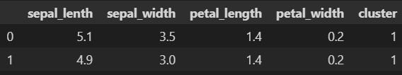

군집 결과 평가를 위한 작업
- yellowbrick : 실루엣 분석을 위한 도구
- pip install yellowbrick

from sklearn.metrics import silhouette_samples, silhouette_score

avg_value = silhouette_score(iris.data, iris_df['cluster'])
score_values = silhouette_samples(iris.data, iris_df['cluster'])

print('avg_value : ', avg_value)
print('silhouette_samples( ) return 값의 shape : ', score_values.shape)

실루엣 plot 결과

from yellowbrick.cluster import silhouette_visualizer

silhouette_visualizer(kmeans, iris.data, colors='yellowbrick')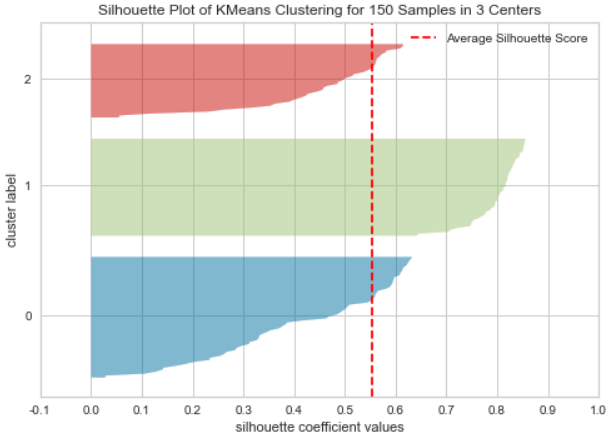

◾군집을 이용한 이미지 분할

1. 이미지 분할(Image Segmentation)

- 이미지 분할

이미지 분할(image segmentation)
- 이미지 분할(image segmentation) : 이미지를 여러 개로 분할하는 것
- 시멘틱 분할(semantic segmentation) : 동일 종류의 물체에 속한 픽셀을 같은 세그먼트로 할당
- 시멘틱 분할에서 최고의 성능을 내려면 CNN 기반이 필요하다
- 색상 분석 시도

- 이미지 읽기

from matplotlib.image import imread

image = imread('ladybug.jpg')
image.shape

plt.imshow(image);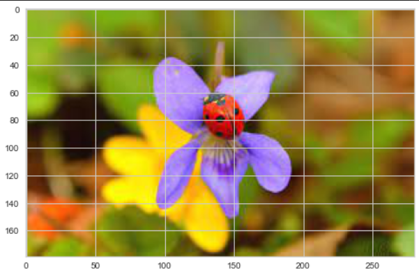

- 색상별 클러스터링

from sklearn.cluster import KMeans

X = image.reshape(-1, 3)
kmeans = KMeans(n_clusters=8, random_state=13).fit(X)
segmented_img = kmeans.cluster_centers_[kmeans.labels_]
segmented_img = segmented_img.reshape(image.shape)

plt.imshow(segmented_img.astype('uint8'));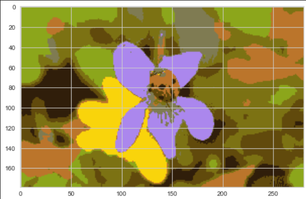

- 여러개의 군집 비교

segmented_imgs = []
n_colors = [10, 8, 6, 4, 2]

for n_clusters in n_colors:
    kmeans = KMeans(n_clusters=n_clusters, random_state=13).fit(X)
    segmented_img = kmeans.cluster_centers_[kmeans.labels_]
    segmented_imgs.append(segmented_img.reshape(image.shape))
plt.figure(figsize=(10, 5))
plt.subplots_adjust(wspace=0.05, hspace=0.1)

plt.subplot(231)
plt.imshow(image)
plt.title('Original image')
plt.axis('off')

for idx, n_clusters in enumerate(n_colors):
    plt.subplot(232 + idx)
    plt.imshow(segmented_imgs[idx].astype('uint8'))
    plt.title('{} colors'.format(n_clusters))
    plt.axis('off')

plt.show()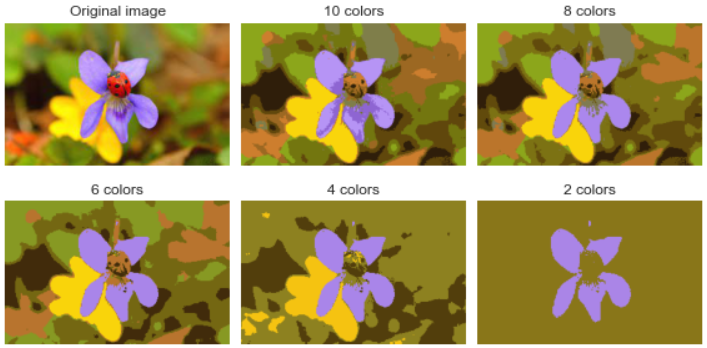

2. MNIST 데이터

- mnist 데이터 읽기

from sklearn.datasets import load_digits
from sklearn.model_selection import train_test_split

X_digits, y_digits = load_digits(return_X_y=True)
X_train, X_test, y_train, y_test = train_test_split(X_digits, y_digits, random_state=13)

X_train.shape, X_test.shape

y_train.shape, y_test.shape

- 로지스틱 회귀

다중 분류이기에 multi_class='ovr' 사용
데이터가 크기 때문에 solver='lbfgs' 사용

from sklearn.linear_model import LogisticRegression

log_reg = LogisticRegression(multi_class='ovr',
                             solver='lbfgs', max_iter=5000, random_state=13)
log_reg.fit(X_train, y_train)

결과는 나쁘지 않다.

log_reg.score(X_test, y_test)

- KMEANS 테스트

전처리의 느낌으로 KMEANS 사용
- 약간 상승하는 것 확인

from sklearn.pipeline import Pipeline

pipeline = Pipeline([
    ('kmeans', KMeans(n_clusters=50, random_state=13)),
    ('log_reg', LogisticRegression(multi_class='ovr', solver='lbfgs', max_iter=5000, random_state=13))
])

pipeline.fit(X_train, y_train)
pipeline.score(X_test, y_test)

- Gridsearch

from sklearn.model_selection import GridSearchCV

param_grid = dict(kmeans__n_clusters=range(2, 100))
grid_clf = GridSearchCV(pipeline, param_grid=param_grid, cv=3, verbose=2)
grid_clf.fit(X_train, y_train)