Geometrical Transforms

파워·2024년 11월 4일

의학영상처리

목록 보기

2/10

Interpolation

Interpolation 이란?

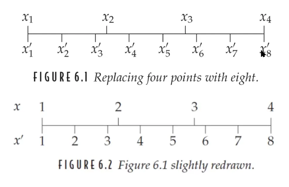
4개의 $x$ 좌표가 있다고 가정하자. 이것을 8개로 늘리고 싶다면 $x1$ 의 값은 그대로지만 나머지 값들은 아닐 것이다. 이를 어떻게 처리해야할까? Interpolation 을 해야한다.

Interpolation 이란 이미지를 확대하거나 축소할 때, 원래의 픽셀 값을 새 위치에 맞추어 새 픽셀 값을 계산하는 과정이다. 간단히 말해, 원래의 픽셀들이 없는 위치에 값을 채워 넣는 기술로, 이미지의 품질을 유지하면서 크기를 조정할 수 있게 해준다.

Interpolation 의 종류

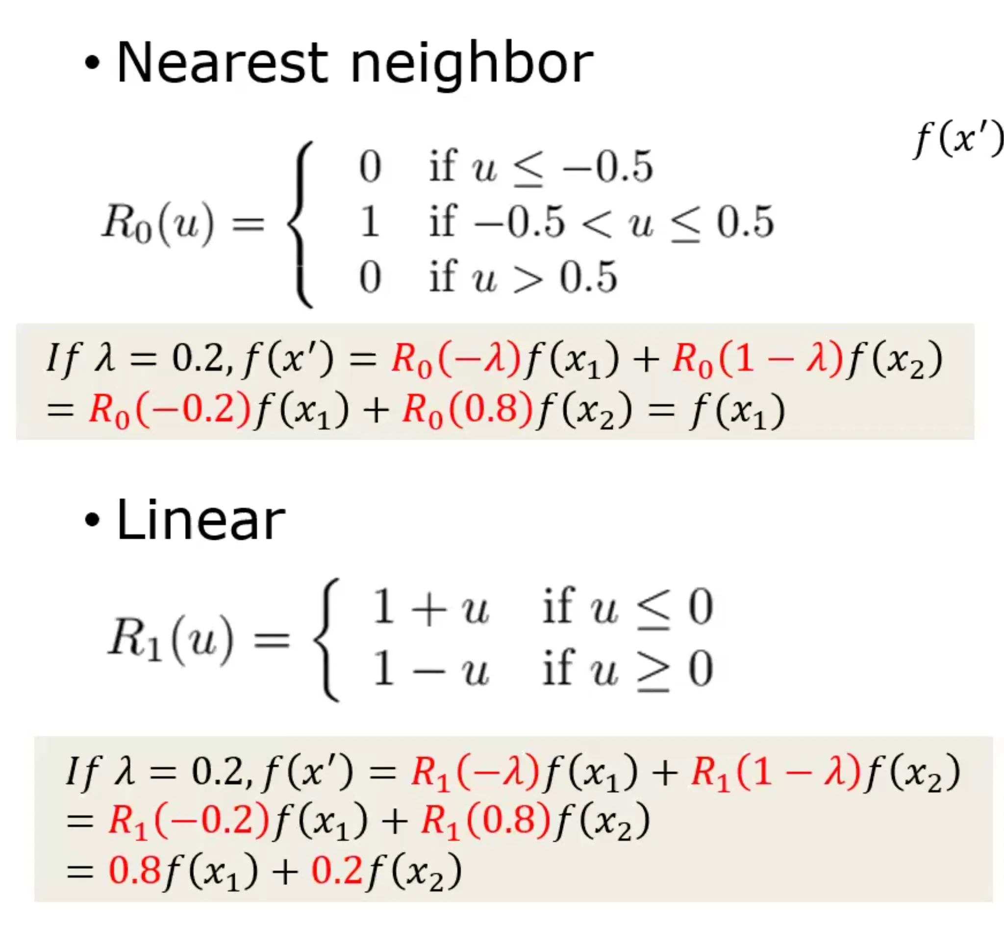
Nearest Neigbor Interpolation

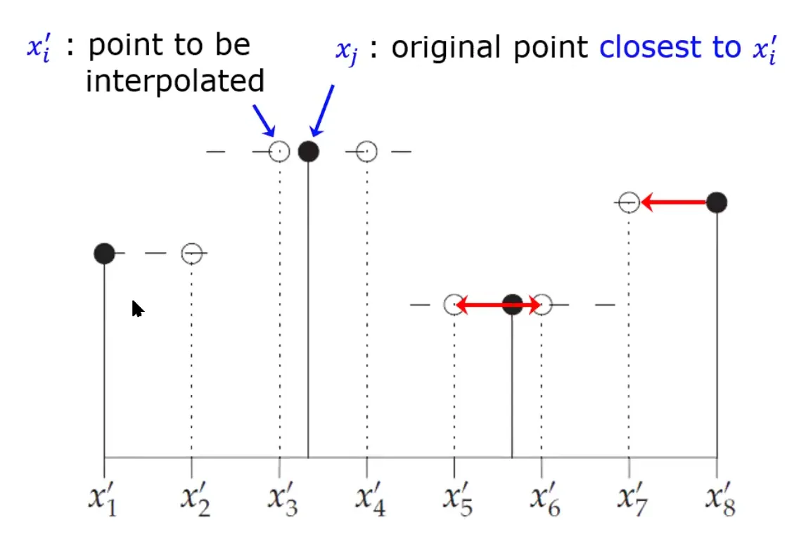
가장 간단한 interpolation 방법이다. 검은 점은 원래 점 $x$ , 흰 점은 interpolation 결과인 $x'$ 점들이다. $x'$ 은 가장 가까운 $x$ 의 값으로 결정한다. 즉,
$x1'=x1$ ,
$x2'=x1$ ,
$x3'=x2$ ,
$x4'=x2$ ,
$x5'=x3$ ,
$x6'=x3$ ,
$x7'=x4$ ,
$x8'=x4$ ,
이다.

Linear Interpolation

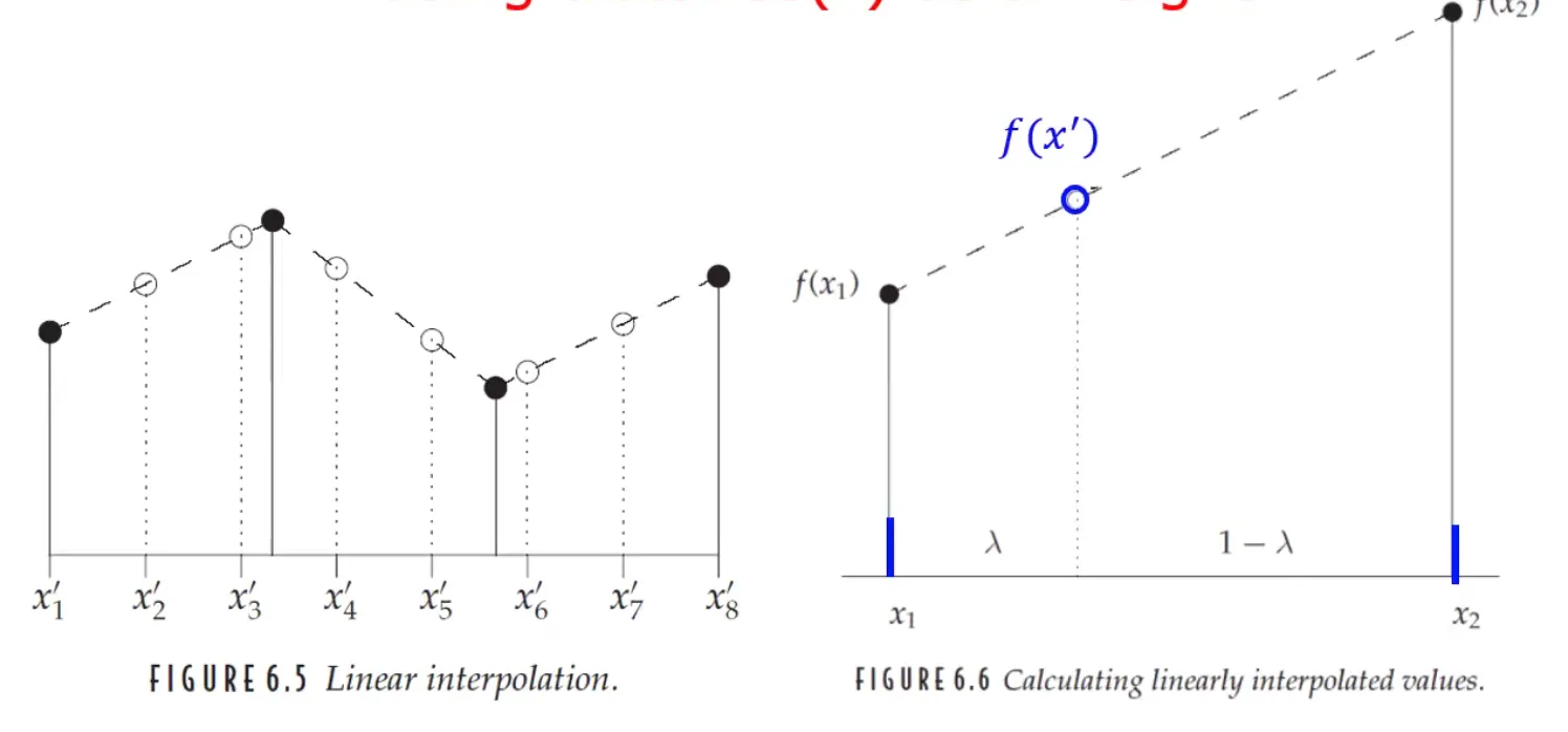
좌우에 이웃한 두 점 사이의 거리 ratio 를 계산해서 $x'$ 를 결정한다. Linear function 그래프를 그린다고 생각하면 편하다.

Bilinear Interpolation

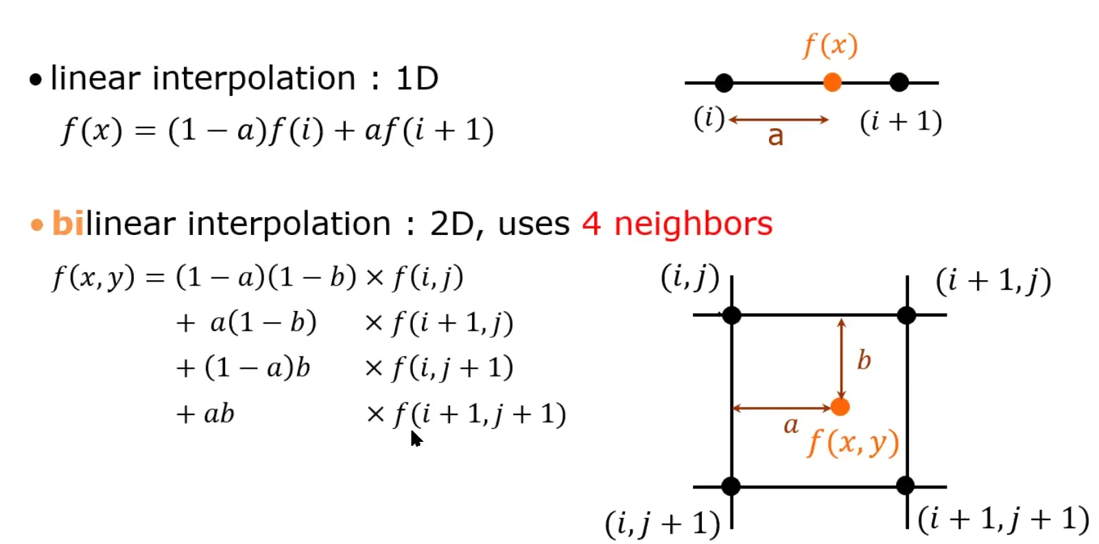
2D array 에서 linear interpolation 을 한다고 생각하면 된다. 주변 4개의 점에 가중치를 계산해서 $f'$ 를 결정한다.

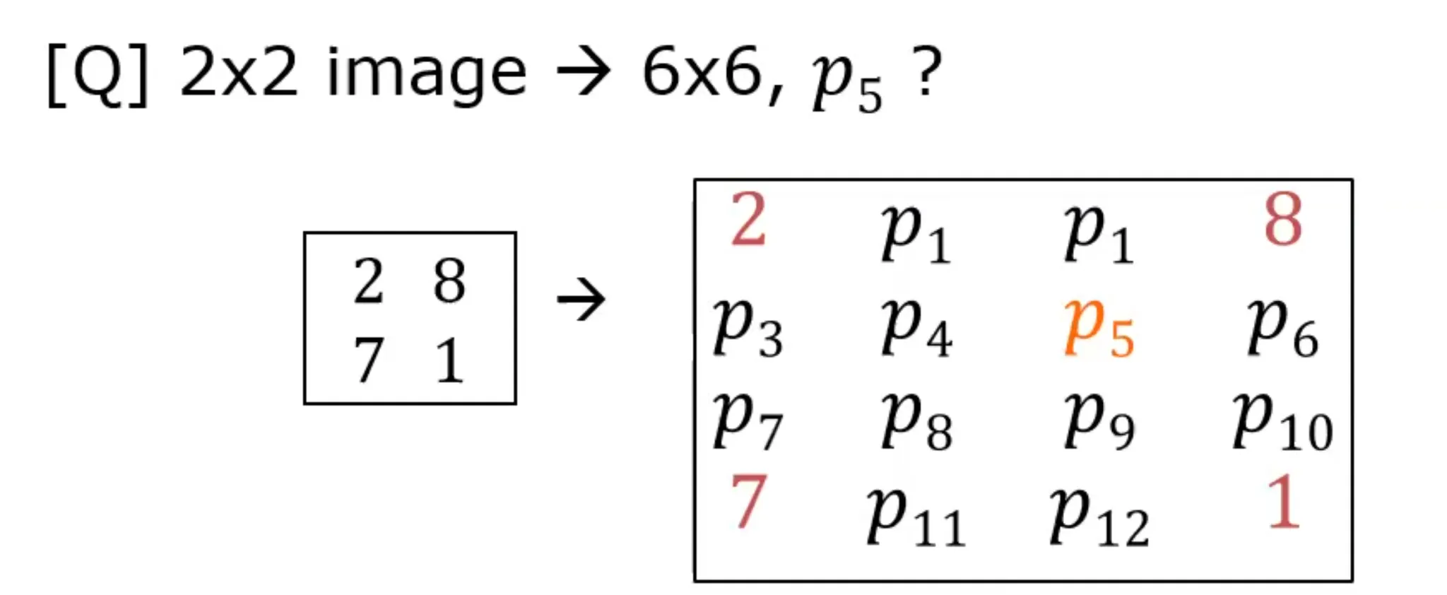
Ans: 5

실제 이미지 파일에서 어떻게 interpolation 이 작동되는지를 이해하는 것이 중요하다. 위의 문제를 직접 풀어보면서 2D array 에서의 interpolation 과정을 이해해보자.

Bicubic Interpolation

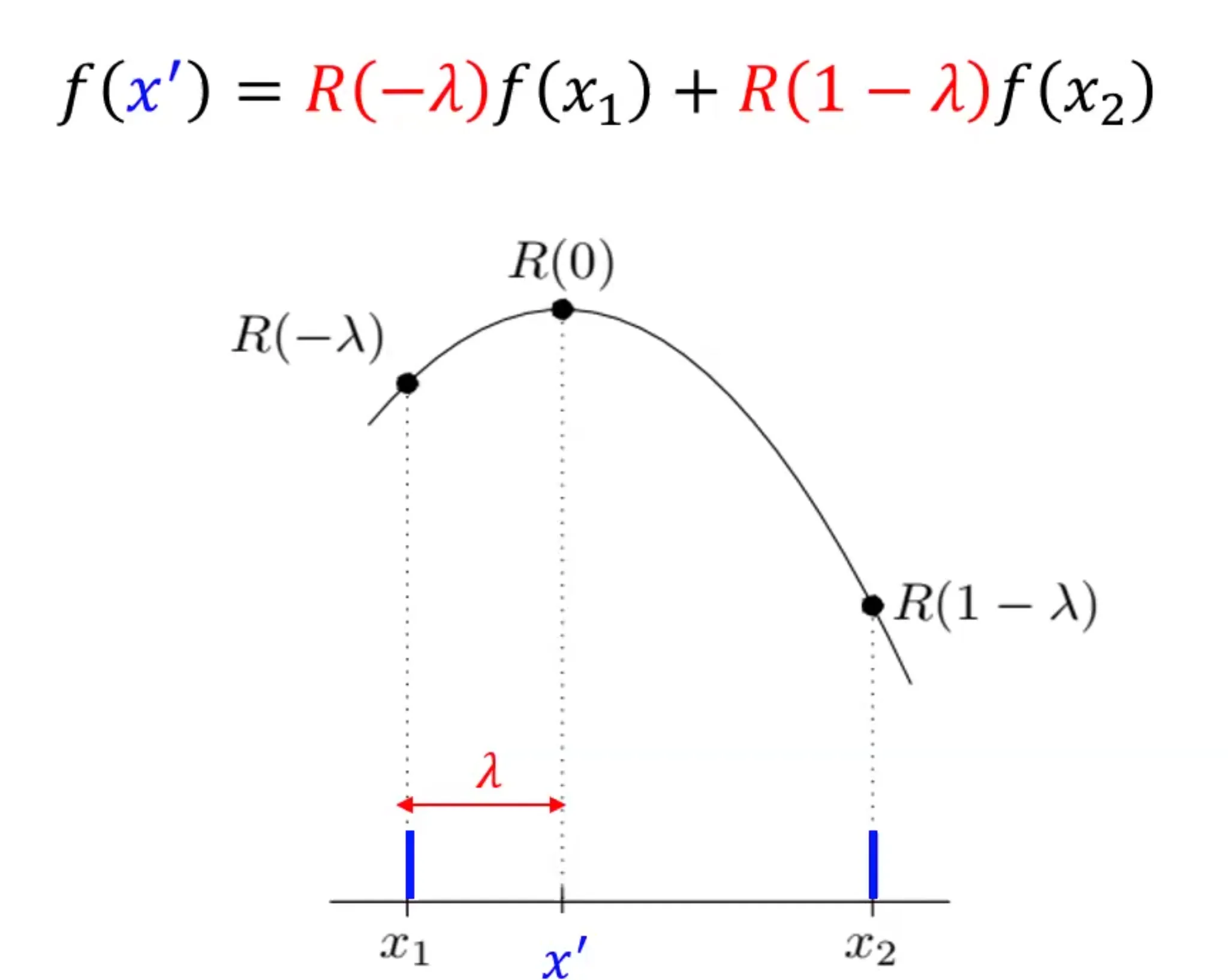
가중치를 계산하는 weight function, $R(u)$ 를 사용해서 $x'$ 를 결정한다. 결과물이 가장 선명하지만 계산량 또한 가장 많다. 컴퓨터의 연산량이 많아 속도가 느리므로 실습에서는 선호하지 않는다.

위 수식처럼 nearest neighbor interpolation, linear interpolation 도 bicubic interpolation 의 방법으로 표현할 수 있다.

Interpolation 구현

skimage.transform.rescale(image, scale, order=1)

특정 interpolation 방법(order 로 지정)을 적용한 이미지를 반환한다.
image: input image
scale: 배율
order: 0(nearest neighbor), 1(bilinear), 3(bicubic)

import numpy as np
import matplotlib.pyplot as plt
import skimage.transform as tr

camera_man = np.array(Image.open('cameraman.tif')
camera_man_head = camera_man[32:96, 89:153]

# Nearest neighbor interpolation
head1 = tr.rescale(camera_man_head, 2, order=0)
# Bilinear: returns pixel values [0.0 1.0]
head2 = tr.rescale(camera_man_head, 2, order=1) * 255
# Bicubic: returns pixel values [0.0 1.0]
head3 = tr.rescale(camera_man_head, 2, order=3) * 255

plt.figure()

plt.subplot(2, 2, 1)
plt.imshow(cameraman_head_np, cmap='gray')
plt.axis('off')
plt.title('Original head')

plt.subplot(2, 2, 2)
plt.imshow(head1, cmap='gray')
plt.axis('off')
plt.title('Nearest neighbor interpolation')

plt.subplot(2, 2, 3)
plt.imshow(head2, cmap='gray')
plt.axis('off')
plt.title('Linear interpolation')

plt.subplot(2, 2, 4)
plt.imshow(head3, cmap='gray')
plt.axis('off')
plt.title('Bicubic interpolation')

plt.show()

필터 마스크 convolution을 이용한 interpolation 구현

이미지를 그저 2배 키우기 위한 목적이라면 컨벌루션을 이요해 빠르게 확대할 수 있다. 말 그대로 크기를 두 배로 키워서 빈 공간에는 0으로 채워 넣는다. 원본 이미지의 두 배 크기의 np.zeros 를 만든 후, i, j 좌표 모두가 홀수인 곳에만 원래 픽셀 값을 채워넣는다.

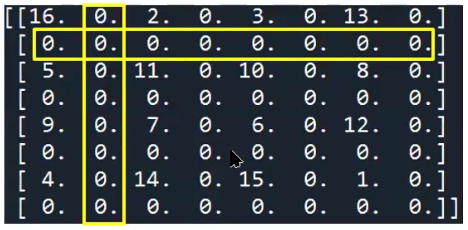
Zero-padded np array

import numpy as np
import scipy.ndimage as ndi

# m: Input image
m = np.array([[16, 2, 3, 13],
              [5, 11, 10, 8],
              [9, 7, 6, 12],
              [4, 14, 15, 1]])
height, width = m.shape
# Input image 의 2배 사이즈의 np.zeros 생성
m2 = np.zeros((2 * hegith, 2 * width))
# np.zero 에서 i, j 좌표가 모두 홀수인 곳에만 input image의 pixel value 입력
m2[::2, ::2] = m

그 후 아래의 필터 마스크를 convolution 하면 interpolation 결과물을 얻을 수 있다.

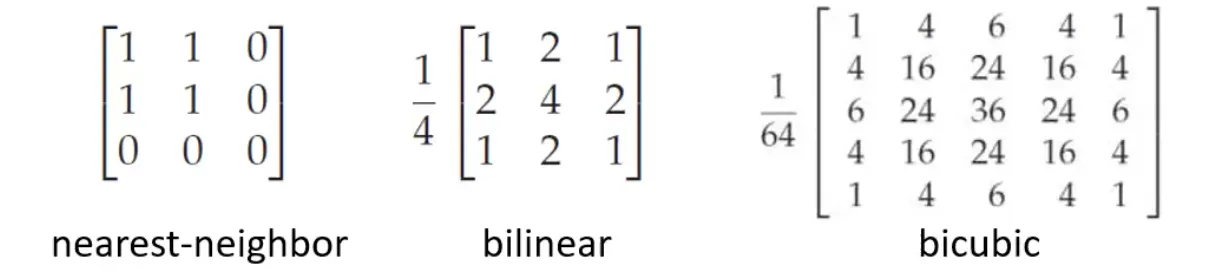
mm1 = ndi.convolve(m2, np.array([[1, 1, 0], [1, 1, 0], [0, 0, 0]]), mode='constant')
mm2 = ndi.convolve(m2, np.array([[1, 2, 1], [2, 4, 2], [1, 2, 2]])/4.0, mode='constant')

print(mm1); print(mm2)

이미지 축소

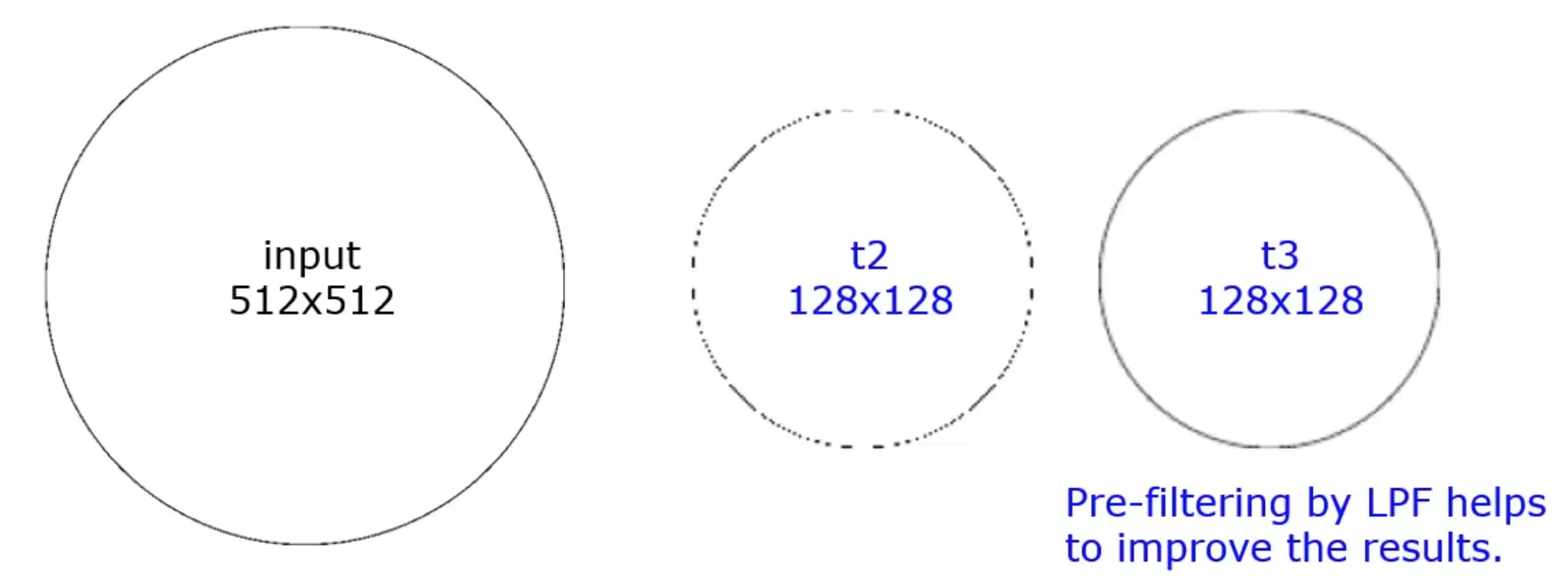
이미지를 함부로 축소시키면 t2처럼 손상된 부분이 생길 수 있다. Bicubic interpolation 로 축소하면 이런 문제를 방지할 수 있다. 미리 LPF 로 필터링하는 것도 좋은 방법이다.

이미지 회전

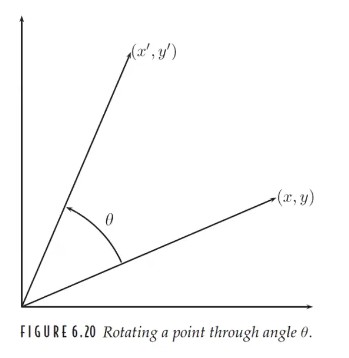
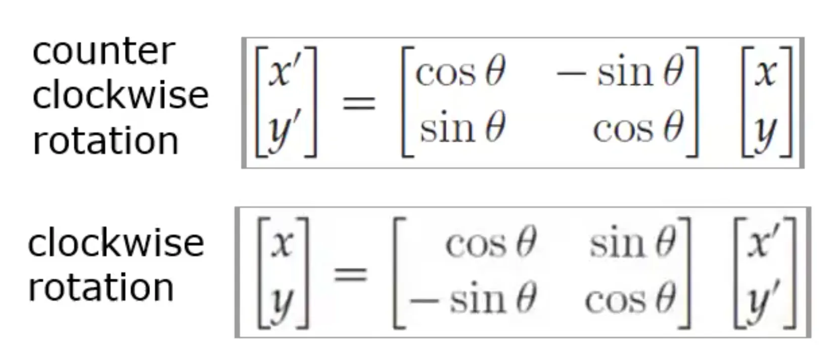
특정 각도로 이미지를 회전하고 싶으면 아래의 공식을 사용하면 된다.

직접 행렬 식을 계산해보면 왜 이런 공식이 도출되었는지 알 수 있을 것이다. 문제는 이 계산의 결과 값이 정수가 아닐 수 있다는 것이다. 또한 회전으로 인해 grid 의 크기가 더 커질 수 있다(이미지는 numpy 배열로 구현되고, 항상 직사각형 모양이기에 grid는 몇몇 특수한 상황을 제외하면 필연적으로 커진다). 아래의 구현 방법을 보면 이 문제점에 대해 더 쉽게 이해할 수 있을 것이다.

이미지 회전 구현

skimage.transform.rotate(image, angle, resize=False, center=None, order=1, mode='constant', cval=0, clip=Ture, preserve_range=False)

angle: 단위는 degree. 시계 반대 방향.
order: 0(neareset neighbor), 1(bilinear), 3(bicubic)
resize: True 는 grid 에 image 가 모두 들어오도록 크기를 resize. False 는 원본 이미지 크기를 유지

import skimage.transform as tr
# 시계 반대 방향으로 60도 회전, nearest neighbor interpolation
# grid 에 image 가 모두 들어오도록 크기를 resize
cr = tr.rotate(c, 60, order=0, resize=True)
# 시계 반대 방향으로 60도 회전, bicubic interpolation
# 이미지의 크기를 유지
crc = tr.rotate(c, 60, order=3)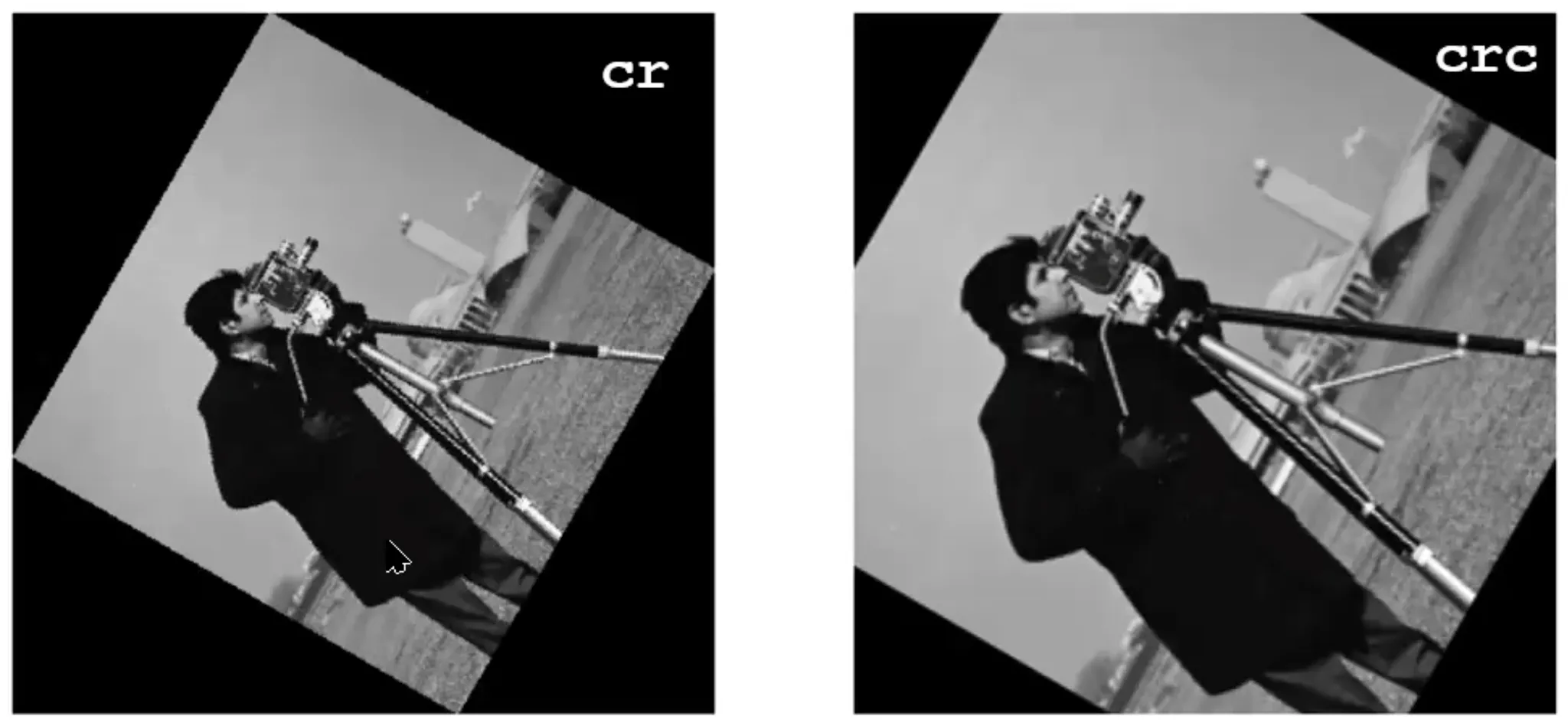

플로팅 된 화면에서는 두 결과 이미지의 크기가 같아 보이지만, 실제로는 cr의 크기가 더 크다(화질을 비교하라). crc는 회전 후 원본 이미지와 pixel size를 유지하기 위해 crop한 것이기 때문에 pixel size는 cr이 더 클 수밖에 없다.

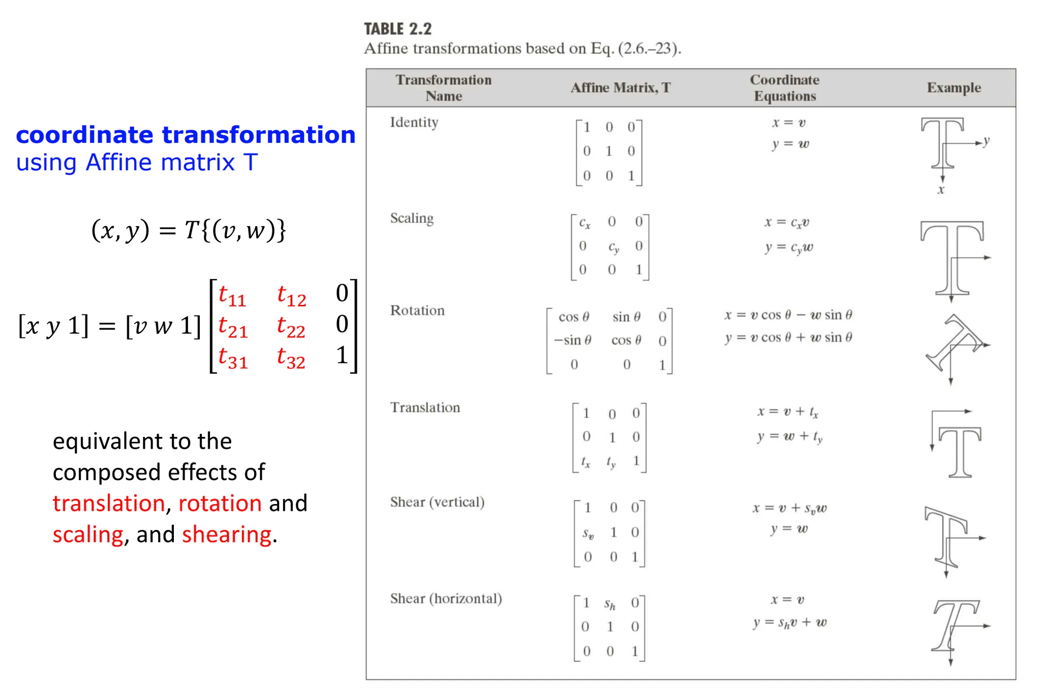
Affine Transform

2D 또는 3D 공간에서 점, 직선 등의 기하학적 객체를 선형 변환과 평행 이동으로 변형하는 방법이다. 이 변환은 직선성을 보존하기 때문에 직선이 곡선으로 바뀌지 않고 평행한 직선은 변환 후에도 평행을 유지한다.

주요 affine transform 에는 다음이 포함된다:

스케일링(Scailing): 이미지를 축을 따라 확대 또는 축소하는 변환으로, $x$ 축과 $y$ 축의 크기를 개별적으로 조정할 수 있다.
회전(Rotation): 객체를 원점이나 특정 기준점을 중심으로 회전시키는 변환.
이동(Translation): 객체를 $x, y$ 좌표로 평행 이동하는 것으로, 위치만 바꾸고 모양이나 크기는 유지한다.
기울이기(Shearing): 축을 따라 눕히거나 기울이는 변화능로, 원래의 직사각형을 평행사변형 형태로 만드는 등 기하학적으로 왜곡.

Affine Transform 구현

skimage.transform.AffineTransform(scale=None, rotation=None, shear=None, translation=None)

Affine transform 행렬을 반환.
scale: (sx, sy), 배율.
rotation: 시계 방향의 회전 각도(단위: 라디안).
shear: (hx, hy), 시계 방향 왜곡.
translation: (tx, ty), 평행이동.

skimage.transform.warp(image, inverse_map, map_args=None, output_shape=None, order=None, mode=’constant’, cval=0.0, clip=True, preserve_range=False)

inverse_map: Affine transform matrix가 들어간다.
order: Interpolation order.
preserve_range: 만약 True 로 설정하면, 입력 이미지 값 범위를 유지한다. 예를 들어 원래 이미지 값이 0 ~ 255 값이라면 이 값이 변한 후에도 유지된다. False 라면 0 ~ 1 범위로 정규화된다.

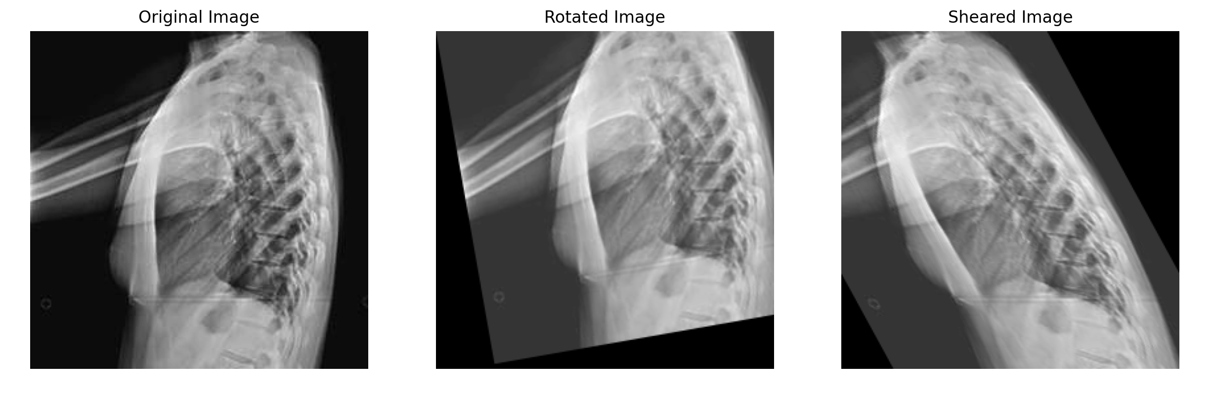
import skimage.transform as tr
import numpy as np
import matplotlib.pyplot as plt
from PIL import Image

image = np.array(Image.open('body.jpg'))

# 회전 각도를 라디안으로 변환
rot = 10 * (3.14159 / 180)

# Affine transformation 정의
tform1 = tr.AffineTransform(rotation=rot)

# 수평 방향으로 0.5 라디안 shear
shr = 0.5
tform2 = tr.AffineTransform(shear=shr, translation=(100, 0))

# 첫 번째 affine transform 실행 (rotation)
rotated_image = tr.warp(image, tform1)

# 두 번째 affine transform 실행 (shear)
sheared_image = tr.warp(image, tform2)

# 결과 이미지 시각화
fig, ax = plt.subplots(1, 3, figsize=(15, 5))

ax[0].imshow(image, cmap='gray')
ax[0].set_title("Original Image")
ax[0].axis('off')

ax[1].imshow(rotated_image, cmap='gray')
ax[1].set_title("Rotated Image")
ax[1].axis('off')

ax[2].imshow(sheared_image, cmap='gray')
ax[2].set_title("Sheared Image")
ax[2].axis('off')

plt.show()