DSP(Discrete Signal Processing) 기본

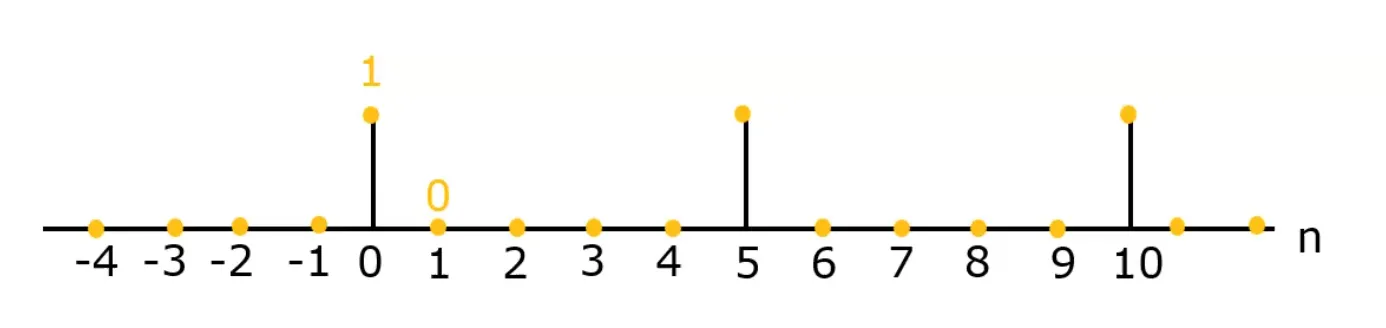
• discrete signal $x[n]$ = {1, 0, 0, 0, 0, 1, 0, 0, 0, 1}
• support of $x[n]$ : {0 ≤ $n$ ≤ 10}
• generalized form of a value of $x$ : $x[n]$
• indexing an element of $x[n]$: $x[0]$ = 1, $x[1]$ = 0, $x[-1]$ = 0

Convolution

---

이미지에서의 convolution

필터의 output signal인 $y[n]$은 input signal인 $x[n]$과 필터의 impulse response인 $h[n]$의 convolution으로 계산된다.

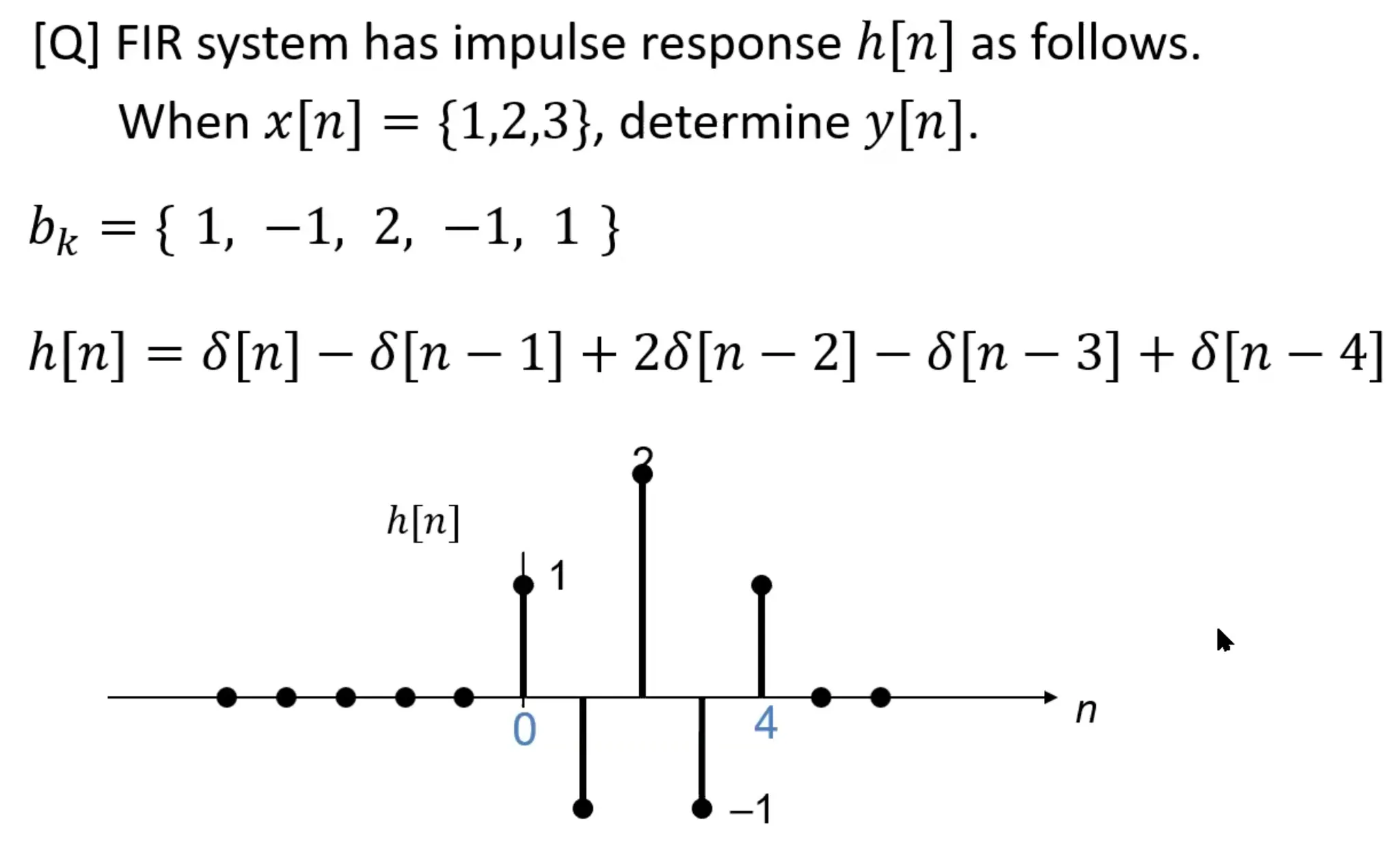
정답: y[n] = {1, 1, 3, 0, 5, -1, 3}

이미지에서는 2D convolution이 기본이다.

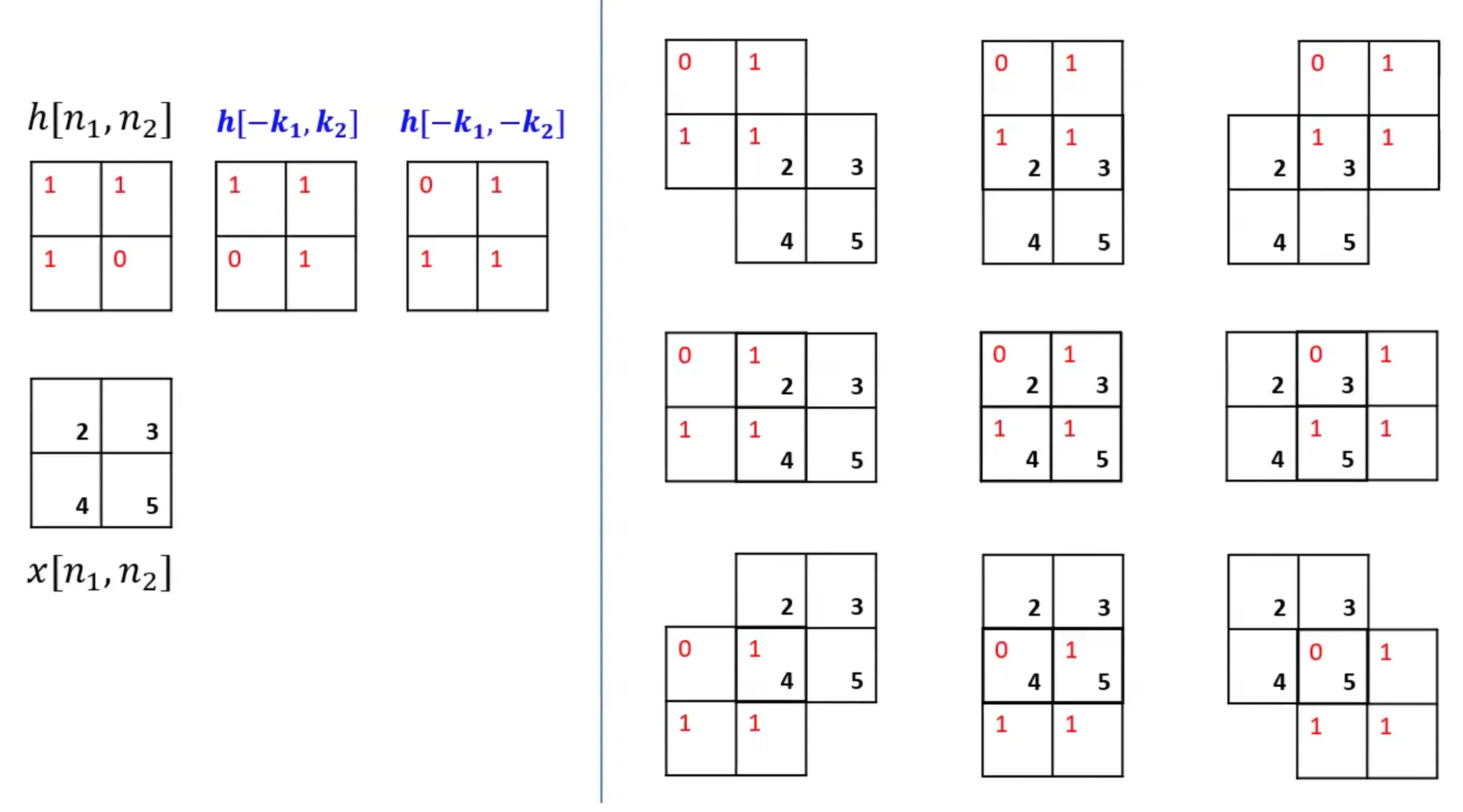
LSI system 에서는 convolution 연산 자체가 neighborhood processing 이고, 그것을 linear filtering 이라고도 부른다.

Convolution 구현

convolve 기본 사용법

scipy.signal.convolve(in1, in2)

• 2개의 1D vector 를 convolution 한다.

scipy.signal.convolve2d(in1, in2)

• 2개의 2D arrays를 convolution 한다.

scipy.ndimage.convolve(input, weights, mode='reflect')

• input과 weights로 필터링 된 이미지를 반환한다. Input array와 같은 size의 이미지를 반환한다.
• input: 2D input arrays $(N * M)$
• weights: 2D filter mask $(M * N)$
• size: $(M + N - 1) ^ 2$
• mode: 'reflect'가 기본값이다. Boundary의 값을 알 수 없으니 내부의 같은 값을 알아서 넣어누즌 것이 reflect다. Boundary를 모두 0으로 넣으려면 'constant'로 하면 된다. 일반적으로 reflect 방법이 선호된다.

import numpy as np
import scipy.signal as sig

# 1D input vector와 filter mask 생성
x1 = np.array([1, 2, 3])
h1 = np.array([1, -1, 2, -1, 1])

# 1D convolution 실행
y1 = sig.convolve(x1, h1); print(y1)
# result: [ 1 1 3 0 5 -1 3]

# 2D input vector와 2D average filter mask 생성
x2 = np.array([[170, 240, 10, 80, 150],
               [230, 50, 70, 140, 160],
               [40, 60, 130, 200, 220],
               [100, 120, 190, 210, 30],
               [110, 180, 250, 20, 90]])
h2 = np.ones((3, 3)) * (1/9)

# 2D convolution 실행
y2 = sig.convolve2d(x2, h2); print(np.uint8(y2))
# result: [[ 18  45  46  36  26  25  16]
#          [ 44  76  85  65  67  58  34]
#          [ 48  87 111 108 128 105  58]
#          [ 41  66 109 130 149 106  45]
#          [ 27  67 131 151 148  85  37]
#          [ 23  56 105 107  87  38  13]
#          [ 12  32  59  50  40  12  10]]

import scipy.ndimage as ndi

y3 = ndi.convolve(x2, h2)
print(np.uint8(y3)); print()

y4 = ndi.convolve(x2, h2, mode='constant')
print(np.uint8(y4))

# y3 result:
#       [[185 132 102  94 135]
#        [136 111 108 128 164]
#        [107 110 130 150 152]
#        [ 95 131 151 148 123]
#        [124 165 157 127  74]]

# y4 result:
#       [[ 76  85  65  67  58]
#        [ 87 111 108 128 105]
#        [ 66 110 130 150 106]
#        [ 67 131 151 148  85]
#        [ 56 105 107  87  38]]

# Boundary에 차이가 있다.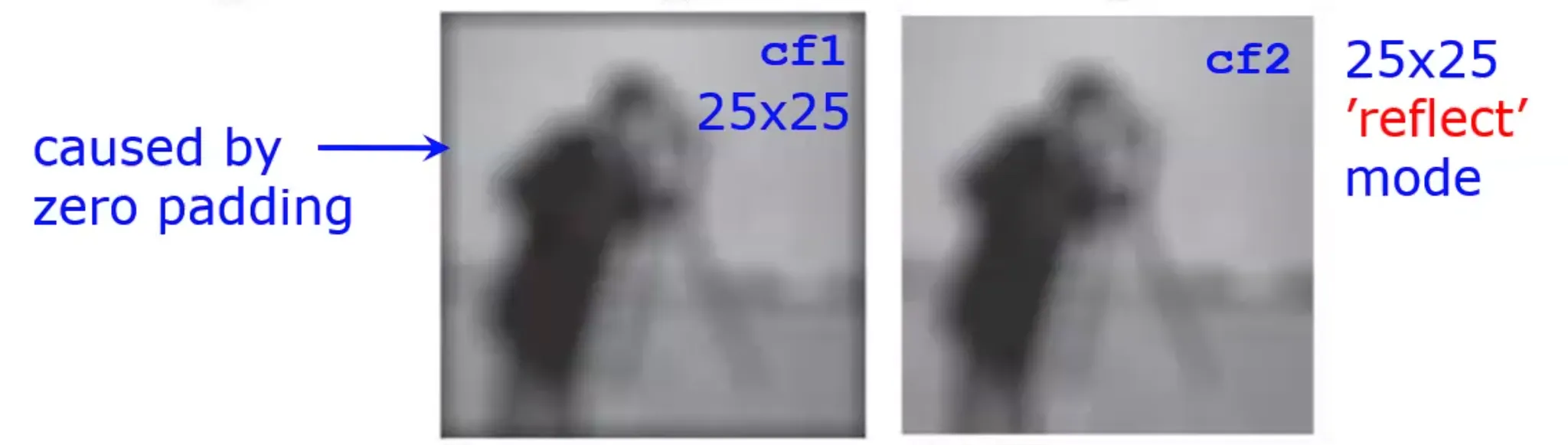

'constant' mode 에서는 모서리가 zero-padding 처리되기 때문에 결과 이미지에 어두운 테두리가 생긴다.

Low-pass filter vs high-pass filter

---

Low-pass filter(LPF)

• LPF는 고주파 성분을 약화시킨다.
• LPF를 사용하면 이미지가 흐려진다.
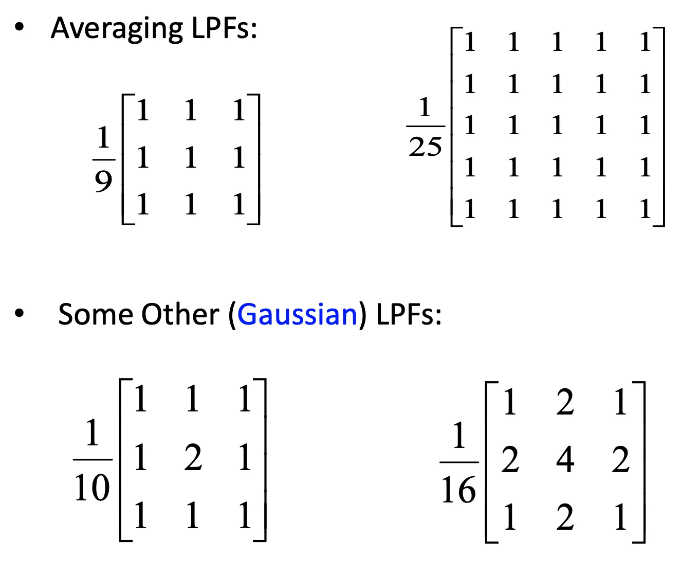
• 대표적인 LPF에는 uniform filter가 있다.

High-pass filter(HPF)

• 이미지 sharpening에 사용된다.
• 고주파 성분을 부스팅한다.
• DC를 제거한다: 밝기 변화가 적은 부분들이 제거된다.

Band-pass filter(BPF)

• LPF 와 HPF 의 tradeoff.

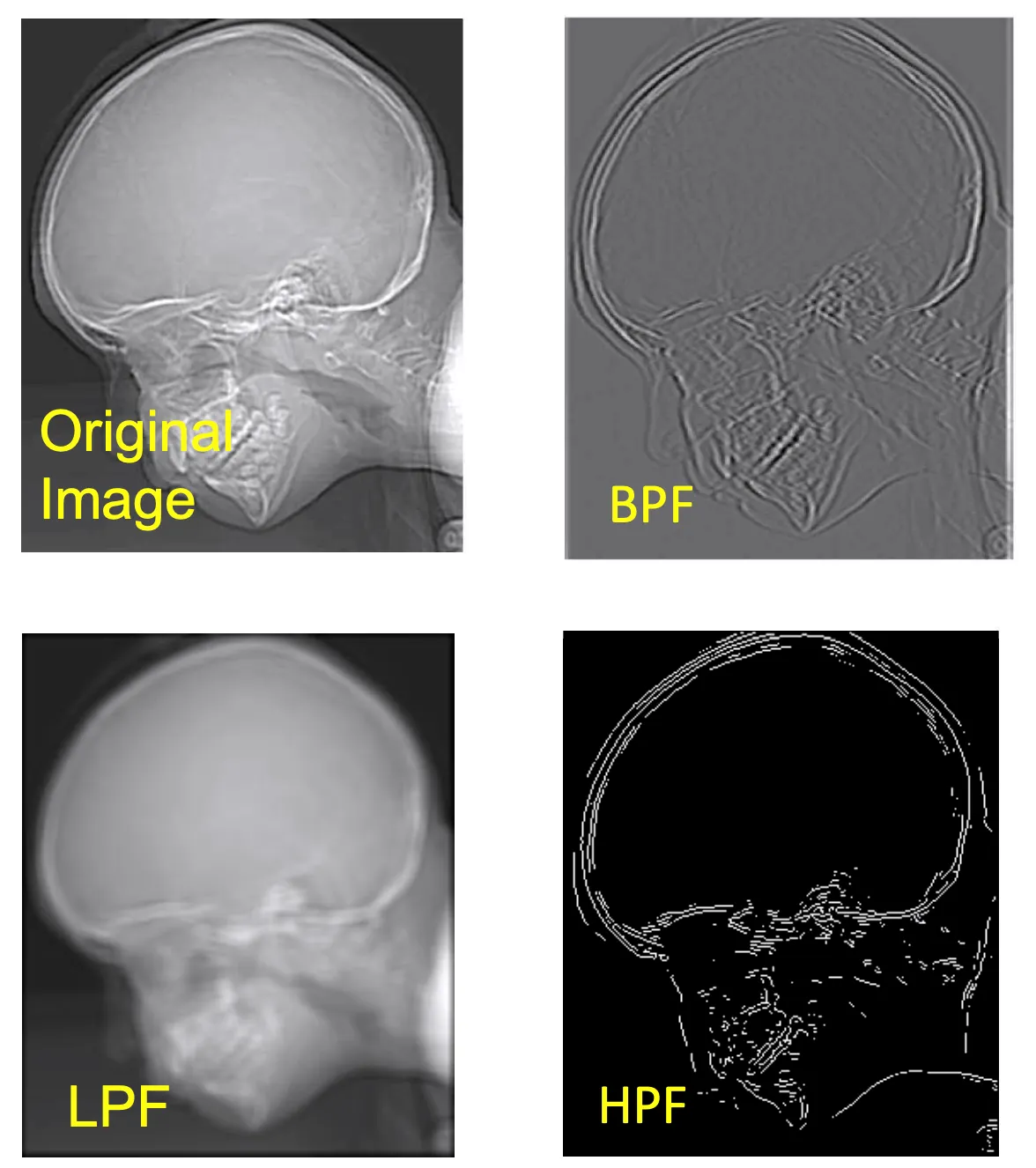
LPF 의 블러링과 HPF 의 DC 제거를 확인할 수 있다.

LPF

---

대부분의 이미지 노이즈는 wideband(e.g. white Gaussian noise)를 가지고 있다. 이것을 억제하려면 LPF 가 필요하다. 주의해야할 점은, LPF 로 저주파대의 노이즈는 제거할 수 없다. LPF 는 블러링을 유발하기 때문에 선명한 경계선을 가진 이미지에서는 치명적이고, 부드러운 대조를 가진 이미지에서는 덜 치명적이다. 따라서 큰 덩어리가 몇 개인지 확인하고 싶을 때 LPF 를 적용해 블러링을 유도할 수 있다. Blocky effect 를 제거하는데도 사용할 수 있는데, 이는 추후에 다루도록 하겠다. LPF 안의 요소들의 합은 1이 되어야 한다.

LPF 는 값들이 무조건 양수로 이루어져있다. 보통 gain을 1로 맞춰주기 위해 추가로 앞에 계수를 붙여준다.

Gaussian filter 구현

scipy.ndimage.gaussian_filter(input, sigma, mode='reflect')

• input: input image
• sigma: sigma value

import numpy as np
import matplotlib.pyplot as plt
import scipy.ndimage as ndi
from PIL import Image

image = Image.open('chest.png')
image_np = np.array(image)

y1 = ndi.uniform_filter(image_np, size=9)    # 9 x 9 평균 필터 적용
y2 = ndi.gaussian_filter(image_np, sigma=3)    # sigma가 3인 가우시안 필터 적용

plt.figure(figsize=(14, 7))

plt.subplot(1, 3, 1)
plt.imshow(image_np, cmap='gray')
plt.title('Input image')
plt.axis('off')

plt.subplot(1, 3, 2)
plt.imshow(y1, cmap='gray')
plt.title('Averaging LPF')
plt.axis('off')

plt.subplot(1, 3, 3)
plt.imshow(y2, cmap='gray')
plt.title('Gaussian filter')
plt.axis('off')

plt.show()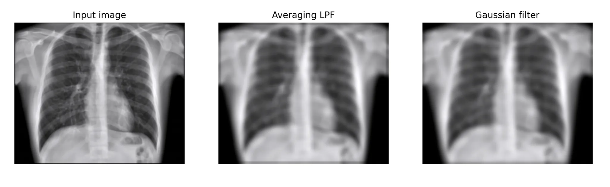

LPF 답게 blurring 된 결과물을 얻었다.

HPF(1차 편미분)

---

LPF는 적분 필터링이라면 HPF는 미분 필터링이다. 1차 편미분 필터는 gradient, 2차 편미분은 laplacian이 명칭 앞에 붙기도 한다.

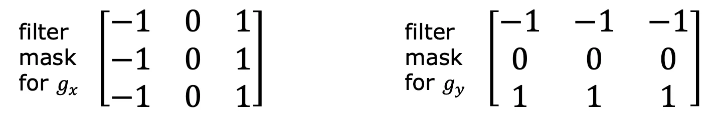
Prewitt filter

1차 편미분(gradient) 필터이다. 수직이나 수평 방향의 미분을 단순한 정수 가중치로 계산한다. 아래는 각각 수직 커널, 수평 커널이다.

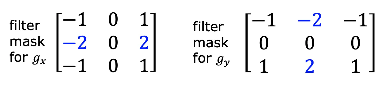
Sobel filter

1차 편미분 필터이다. Prewitt filter와 유사하지만 중심 요소의 가중치가 더 높다. 이는 경계 검출 시 노이즈에 대한 내성을 높이기 위해 설계된 것이다.

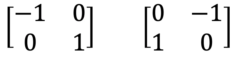
Robert filter

1차 편미분 필터이다. 대각선 edge 정보를 강조하는 필터이다.

필터링 이미지 비교

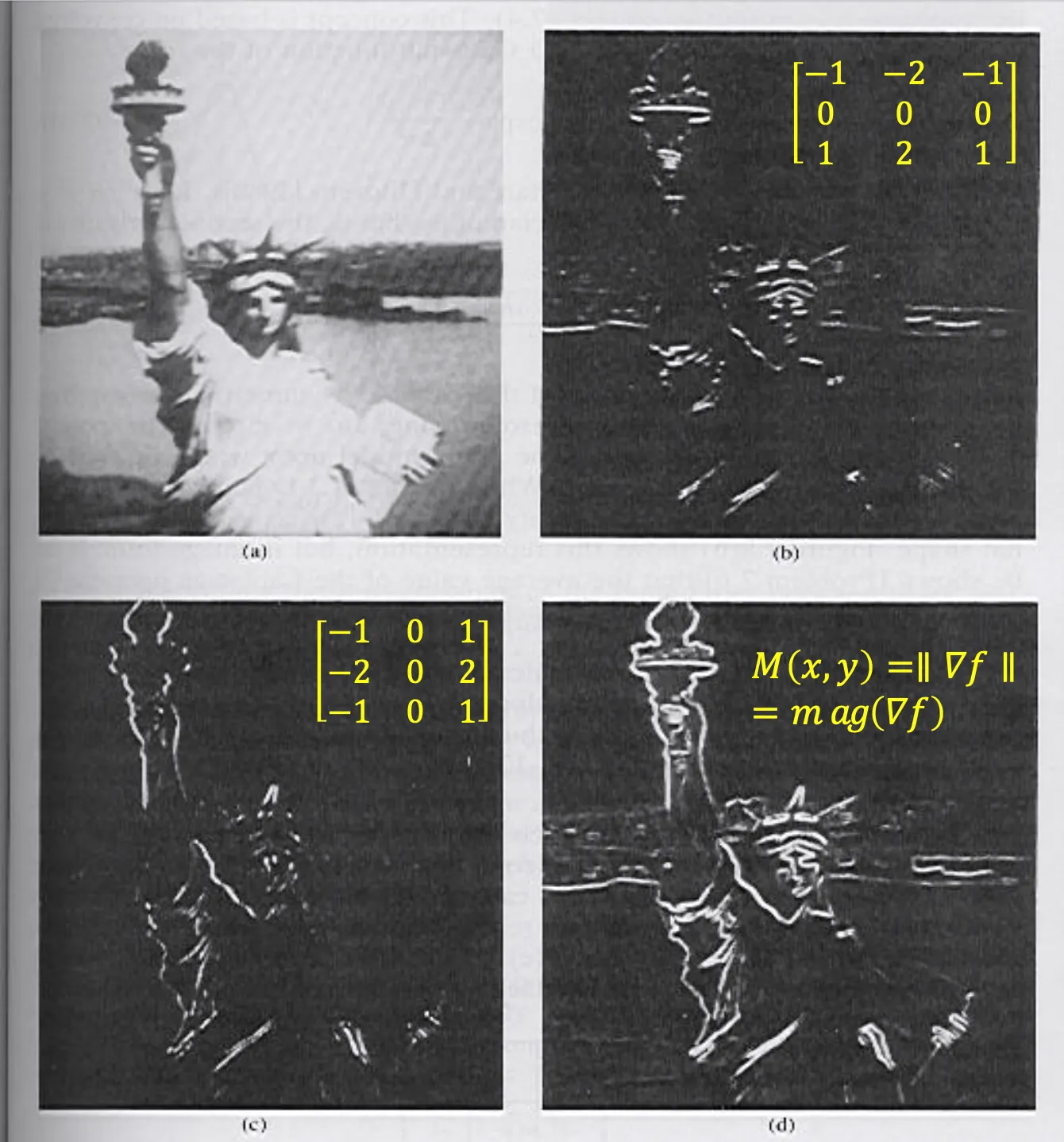
(a) Original image, (b) Sobel filtered image(horizontal edges), (c) Sobel filtered image(vertical edges), (d) magnitude of gradients

HPF(2차 편미분)

---

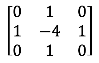
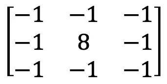
Laplacian filter

• 목적: 이미지의 세밀한 디테일 강화
• 모든 coefficients 의 합은 0이어야 한다! 즉, gain 이 0 이다!

LoG filter

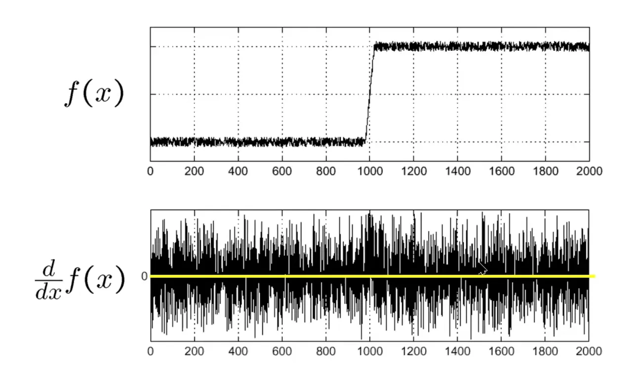
노이즈가 매우 많은 이미지는 한 번 미분을 하더라도 엣지를 찾기 힘들다. 이것이 HPF의 단점이다. 이를 극복하기 위해 어떤 필터를 사용해야할까?

Laplacian of Gaussian. Gaussian filter를 먼저 적용한 다음 laplacian filter를 적용한다. Edge는 분명하지만 Edge 주변이 모두 작은 진폭으로 진동하는 형태라 HPF를 적용했을 때 모든 부분이 강조되는 경우가 있는데, 그것을 방지하기 위한 방법이다. Gaussian filter로 먼저 부드럽게 만들어 줬기 때문에 확실하게 edge의 위치를 찾아낼 수 있다.

1차 편미분 LPF를 먼저 사용하는 경우는 DoG(Derivative of Gaussian) filter라고 부른다.

HPF 를 이용한 이미지 선명화

HPF를 사용한 이미지는 edge부분이 선명하게 나오고 나머지는 어둡게 나온다. HPF 만으로는 이미지를 선명하게 만들 수 없다. 이것을 원본 이미지에 빼면 더 선명한 이미지를 얻을 수 있다.

Median filter

---

LPF를 적용하면 노이즈를 제거할 수는 있지만 블러링이 일어난다. 블러링 없이 노이즈를 제거할 수 없을까? Median Filter를 적용하면 된다.

Median Filter는 non-linear filter이다. 이전까지 살펴본 filter 들은 모두 linear filter(convolution을 통해 계산하는 filter)이다. 이 필터로 salt-and-pepper 노이즈를 제거하면서 edge를 보존시킬 수 있다.

Median filter 구현

scipy.ndimage.median_filter(img, size=n)

• img: input image
• size: 필터의 커널 크기. 예를 들어, size=3이면 3x3 커널이 적용된다. 값이 클수록 더 넓은 영역을 참조하므로 부드러운 효과가 나지만, 디테일이 더 많이 사라질 수 있다.

import numpy as np
import matplotlib.pyplot as plt
from PIL import Image
import scipy.ndimage as ndi

img = np.array(Image.open('sadimg.bmp'))
filtered_img = ndi.median_filter(img, size=3)

plt.figure(figsize=(10, 6))

plt.subplot(1, 2, 1)
plt.imshow(img, cmap='gray')
plt.title('Original image')
plt.axis('off')

plt.subplot(1, 2, 2)
plt.imshow(filtered_img, cmap='gray')
plt.title('Median filtered image')
plt.axis('off')

plt.show()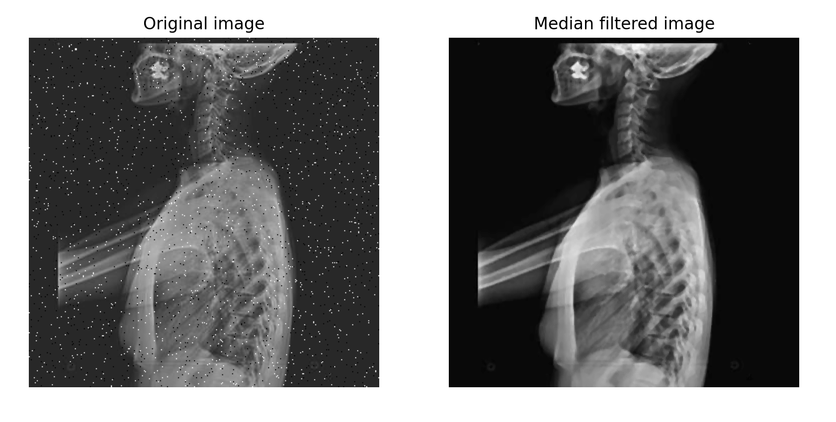

Salt-and-pepper 노이즈가 제거되었다.