Image Processing 3

Sampling and Quantization

object : Generate a digital image from sensed data
목표 : 감지된 데이터로부터 디지털 이미지 생성

the output of the sensors that we get is a continuous voltage waveform.

In order to create a digital image, we need to convert the continuous sensed data into digital form
디지털 이미지를 생성하기 위해, 연속적인 감지된 데이터를 디지털 형태로 바꿔야함.

To do this, we need to have 2 processes : Sampling and Quantization

---

• sampling an analog signal is instantaneously measuring the voltage of the signal at a fixed interval in time(discretization of time)
  아날로그 신호를 샘플링하는 것은 고정된 시간 간격으로 신호의 전압을 순간적으로 측정하는 것

• the value of the voltage of the signal at each instantis converted into a number and stored
  각 순간의 신호의 전압값을 숫자로 변환하여 저장한다.

• The number ths is stored represents the brightness of the image at that point
  저장된 숫자는 그 지점의 이미지의 밝기를 나타낸다.

• the stored number is a digital image that can be accessed as a two dimensional array of data
  저장된 숫자는 데이터의 2차원 배열로 접근할 수 있는 디지털 이미지이다.

• Each Data Point Is Called a Pixel

• 디지털 이미지 표기법 : I(r, c)
  I(r, c)is the brightness of the image at point (r, c)
  I(r, c)는 (row, column) 지점에서의 이미지 밝기

---

Basic concepts in Samppling Quantization

• Let a continuous image f be converted to a digital form

• An image may be continuous with respect to the x and y coordinates and also in amplitude
  이미지는 x, y 좌표와 진폭에 대해 연속적일 수 있다.

• To convert it to digital form, we have to sample the function in both coordinates and in amplitude
  디지털 형식으로 변환하기 위해, 좌표와 진폭에서 함수를 샘플링해야한다.

Digitizing the coordinate values is called sampling
Digitizing the amplitude values in called quntization
좌표 디지털화 = 샘플링
진폭 디지털화 = 양자화

---

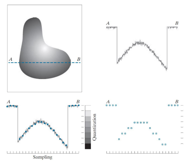
연속 이미지의 진폭값을 AB에 따라 그림.
동일한 간격(equally spaced)으로 샘플을 채취.

• The continuous intensity levels are quantized by assigned one of the eight values to each sample.
  연속 강도 레벨은 8개의 값중 하나에 할당하여 양자화 된다.
• the assignment is made depending on the vertical proximity(근접) of a sample of a vertical tick mark
  수직 눈금 표시 샘플의 수직 근접성에 따라 할당이 이루어진다.
• Starting at the top of the image and carrying out this procedure line by line produces a 2-dimensional digital image
  이미지 상단부터 시작하여 한 줄 씩 수행하면 2차원 디지털 이미지가 생성된다.

In addition to the number of discrete levels used, the accuracy achieved in quantization is highly dependent on the noise content of the sampled signal
정확도는 노이즈의 함량에 따라 크게 달라짐.

그래서 이미지 생성에 사용된 센서 배열에 따라 샘플링 방법이 달라짐.

mechanical motion과 결합된 single sensing element에 의해 이미지가 생성되면 위와 같은 방식으로 양자화됨.

---

• When a sensing strip is used for image acquisition, the number of sensors in the strip establishes the sampling limitations in one image direction
  감지 스트립을 사용하는경우, 스트립 센서 수에 따라 샘플링 제한이 설정 됨. (한 방향)

• when a sensing array is used for image acquisition, there is no motion and the number of sensors in the array establishes the limits of sampling in both directions.
  감지 어레이를 이미지 획득에 사용하는 경우, 움직임이 없고 센서 수에 따라 양방향 샘플링 한계가 설정됨

  Quantization will be as before. 양자화는 이전과 같음

The more number of steps or sensors (+intensity levels) -> more quality sampling and quantization

더 많은 스텝/센서/개별 강도 -> 더 나은 품질의 샘플링/양자화

---

Representing Digital Images

• Let f(s, t) represent a continuous image function of two continuous variables
• Supprose that we sample the contiuous image into a 2D array, f(s,t), containing M rows and N columns, where (x,y) are discrete coordinates

  x = 0,1,2,..., M-1
  y = 0,1,2,..., N-1

There are three basic ways to represent f(x,y)

First

• Plot of the function with two axes determining spatial location and the third axis being the values of (intensities) as a function of the two spatial variables x and y
  공간을 결정하는 두 개의 축(x,y), x와 y의 함수이자 f(강도) 값인 세 번째 축이 있는 함수
• 이 representation은 gray-scale 작업에 유용함

Second

• f(x,y) as it would appear on a monitor or photographer
  모니터나 사진처럼 표현
• if intensity is normalized to the interval [0,1], then each point in the image has the value 0, 0.5, 1
  강도가 [0,1]로 정규화되면 이미지의 각 지점은 0, 0.5, 1의 값을 가짐
• much more common

Third

• display the numerical values of f(x,y) as an array(matrix)
  세번째 표현은 단순히 f(x,y)의 수치를 배열(행렬)로 표시하는 것
• f is of size 600X600 elements -> 360000 numbers
• quite useful when only parts of the image are printed and analyzed as numerical values
  이미지의 일부만 인쇄하여 분석하는 경우에는 이 표현이 유용

Mathematical modeling of Images

• Each element of matrix is called an pixel
• The origin of a digital image is at the top left
• There are no restirctions on M, N, other than they have to be positive
• intensity levels typically is an integer power of 2 (L = 2^k)
• we assume that the discrete levels are equally spaced and that they are integers in the interval [0, L-1]

---

Spatail(공간적) and Intensity Resolution(밝기 해상도)

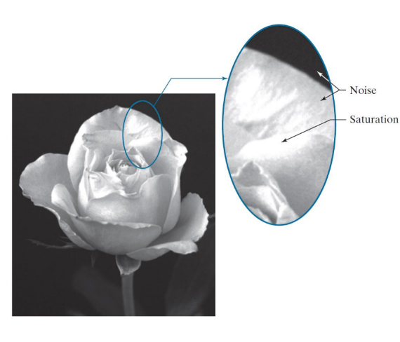
Sturation(포화) is the highest value beyond which all intensity levels are clipped

clipping : 일정 수치 이상 올라가면 잘라냄. 사진에서 하얀색 부분

• Noise in this case appears as a grainy texture pattern
• Noise mask the lowest detectable true intensity level

spatail resolution is a measure of the smallesst discernible detail in an image 공간 해상도는 이미지에서 식별할 수 있는 가장 작은 세부사항을 측정한 것이다.

spatial resolution 은 다양한 방법으로 설명할 수 있다.
1. dots(pixel) per unit distance : 단위 거리당 픽셀
2. DPI (= dots per inch) : 인치당 픽셀
3. line pairs per unit distance

intensity resolution similarly refers to the amllest discernalble change in intensity level

밝기 해상도는 intensity(밝기) level에서 식별가능한 가장 작은 변화를 나타낸다

Unlike spatial resolution, it is common to refer to the number of bits used to quantize intensity as the intensity resolution
intensity를 양자화 하는데에 사용되는 비트수를 intensity resolution으로 하는 것이 일반적이다.

---

Image Detail

Detail can be described as information as an image is considered a signal

interpolation(보간법) is basic tool used in tasks such as zooming, shrinking(줄어들다), rotating, geometric corrections.

• 보간법은 주위 화소들로부터 하나의 화소 값을 결정하는 것

Principal objective is image resizing(shrinking and zooming), which are basically image reampling methods

interpolation is the process of using known data to estimate values at unknown location

interploation은 알려진 데이터를 사용하여 알려지지 않은 위치의 값을 추정하는 것.

Nearset Neighbor Interpolation

An image of size 500X500 pixels has to be enlarged 1.5 times to 750X750 pixels.

• A simple way of visualize zooming:

1. Create the imaginary 750X750 grid with the same pixel spacing as the original,
2. and then shrink it so it fits over the original image
   원본과 동일한 픽셀 간격으로 가상의 750X750 그리드를 만든 다음, 원본 이미지에 맞도록 축소
3. intensity-level assignment is performed by assigning intensity of its closest pixel in the original image to the new pixel in the 750X750 grid
   원본이미지에서 가장 가까운 픽셀의 intensity를 750X750 그리드의 새 픽셀에 할당하여 intensity-level assignment 수행
4. After intensity-level assignment, expand it to the original specified size to obtain the zoomed image
   원래 지정된 크기로 확장하여 확대된 이미지를 얻는다.
   축소된 750X750 그리드는 원본 이미지의 픽셀 간격보다 작다.
   
   

Method is called Nearset Neighbor Interpolation

: Assings to each new location the intensity of its nearset neighbor in the original image, 원본 이미지에서 가장 가까운 이웃의 intensity를 각 새 위치에 할당
this Method has the tendency to produce undesirable artifacts, such as severe distortion of straight edges.

-> Used Infrequently

Bilinear Interpolation

• More suitable.

Use of the four nearest neighbors to estimate the intensity at a given location

4개의 가장 가까운 이웃을 사용하여 intensity 추정

• Assigned value
  v(x, y) = ax + by + cxy + d

Bilinear interpolation gives better results than nearest neighbor interpolation, with a increase in computational burden

Bicubic interpoloation

: involves the sixteen nearest neighbors of a point

• Assigned value
  
• sixteen coefficients are determined from the sixteen equations in sixteen unknowns

bicubic interpolation does better job of preserving fine detail than its bilinear counterpart at the expense of computational complexity

일반적으로 bicubic은 bilinear보다 더 계산이 복잡하지만, 세부사항을 더 보존하는 더 나은 작업을 수행한다.

• using more neighbors in interpolation offers more complex techniques and can yield better results
• preserving fine detail is important image generation for 3-D