[Paper]Topological GNNs

TOPOLOGICAL GRAPH NEURAL NETWORKS
https://arxiv.org/pdf/2102.07835.pdf

Topological Graph Layer (TOGL)은
Topological data analysis(TDA) 기반의 layer이다,
persistent homology를 이용해서 그래프의 global topological information을 고려하는 layer 이다.
Weisfeiler-Lehman graph isomorphism test (WL test) 면에서 message-passing GNNs(MPNN)보다 낫고 모든 종류의 GNN에 쉽게 적용될 수 있다.

WL test : https://process-mining.tistory.com/170
TDA : https://velog.io/@shlee0125/TDA%EC%9D%98-%EA%B8%B0%EC%B4%88-02-Homology

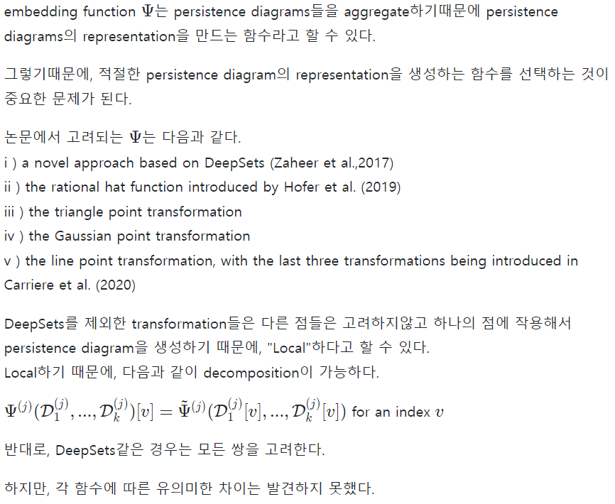
해당 논문의 motivation이 되는 예시는 다음 그림과 같다.

왼쪽같은 cycles graph는 topology based method로 쉽게 구분할 수 있다.
해당 사실을 GCN-TOGL & PH(a method based on static topological features)가 적은 iteration으로 금방 높은 성능을 보인다는 사실을 통해 알 수 있다.

오른쪽같은 necklaces graph는 learnable topological features가 필수적인 형태이기 때문에 해당 논문에서 제시하는 TOGL layer를 적용한 GCN이 높은 성능을 보인다.

Background : computational topology

...
https://en.wikipedia.org/wiki/Homology_(mathematics)
https://en.wikipedia.org/wiki/Betti_number

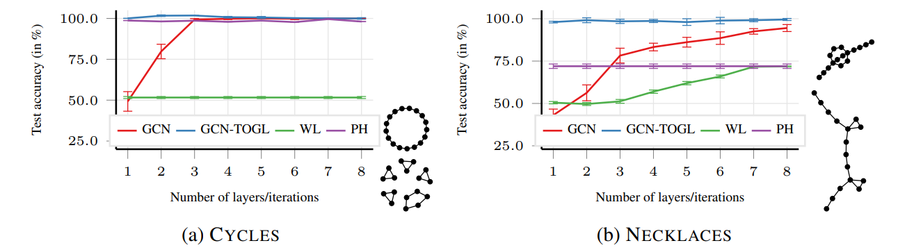
Overview of the components of TOGL

overview schematic의 input과 ouput을 보면 알 수 있듯이 기존의 GNN에 쉽게 추가 가능한 형태이다.

input graph $G = ( V, E )$ $V$에는 n개의 노드들이 있고 edge들의 집합을 $E$이라고 한다.

각각의 node $v$에는 d 차원의 node attribute가 있다.
다시말해서 node attribute $x^{(v)} \in V$ 이다.

$x^{(v)}$는 data의 node features에 해당한다고 말할 수도 있고 GNN에 의해서 학습되는 hidden representation이라고도 할 수 있다.

(a) $x^{(v)} \in \mathbb{R}^{d}$ : 차원 d인 node attribute vector

(b) $\Phi$ : $x^{(v)}$를 k개의 node "value" $a^{v}_{1} ,..., a^{v}_{k}$($\in\mathbb{R}$, 각각) 로 mapping하는 함수

(c) 각각의 vertex v의 attribute, $x$에 $\Phi_k$를 적용한다.
k개의 view of graph $G$가 생긴다.

(d) 각각의 $i$th view of $G$에서 filtration $f_i$를 계산한다.
vertex filtration function $f_i :\mathbb{R}^{d} \rightarrow \mathbb{R}, i =1,... ,k$
각각의 $f_i$를 통해 그래프의 다양한 properties를 고려하게된다.

(e) $f_i$를 통해 Persistence diagram들을 생성한다.
vertex v에서 시작해 생성된 모든(k개) persistence diagram들은 embedding function $\Psi[v]$를 통해 embedding된다. : embedded topological features라고 부르자.

(f) embedded topological features는 input attribute $x^{(v)}$와 합쳐진다. 그렇게 합쳐진 결과를 $\tilde{x}^{(v)}$라고 하자.

(g) 마침내, topological information을 고려한 new node representation $\tilde{x}^{(v)} \in\mathbb{R}^d$ 을 얻는다.

filtration function $f_i$를 통해 $l$개의 Persistence diagrams을 구성하고
embedding function $\Psi^{(l)}:{\{D^l_1, ... , D^l_k \rightarrow \mathbb{R}^{n^{'}\times d}}\}$를 통해서 embedding 한다.

$l$ 같은 경우는 처음에는 단순화를 위해 $l = 1$인 경우, 즉 하나의 $f_i$을 통해서 하나의 Persistence diagram을 생성하는 경우를 묘사한다. 논문에서 후술하는 정리를 통해서 복수의 $l$에 대해서 일반화가 가능하다는 증명을 하게된다.

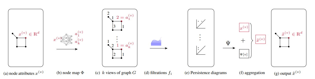
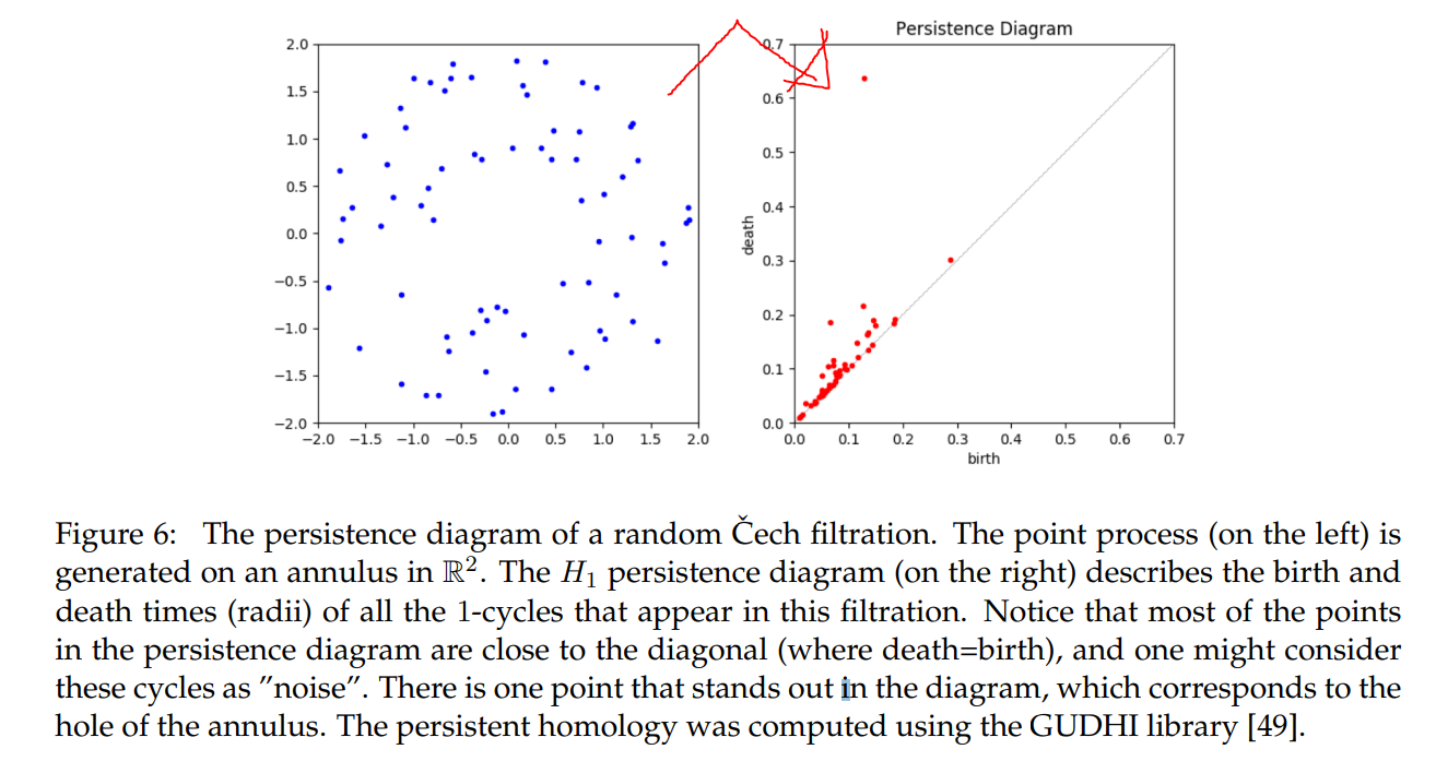
persistence diagram: for example)

https://www.researchgate.net/publication/265730257_Topology_of_random_geometric_complexes_a_survey

Details on filtration computation and output generation.

filtration function $f_i$는 single hidden layer를 갖는 MLP이다.
즉, $f_i := \pi_i \circ\Phi$ 라고 node map $\Phi$를 고려해서 표현할 수 있다.
이러한 맥락에서, $\Phi$는 $x^{(v)}$의 hidden representation을 위한 mapping이라고 할 수 있다.

$f_i$의 결과로 persistent diagram을 얻으며, $\Psi^{(0)}$를 통해 각각의 persistent diagram들을 aggregate 하고 original node attribute인 $x^{(v)}$와 더해서 "topological embedding of vertex $v$"를 얻게되는데,

original node attribute와 더한다는 점에서 "residual fashion"이라고 표현할 수 있다.

! 더 자세한 논의를 위해선 persistent diagram의 이해가 선행되어야함 !

Complexity and limitations

1. d-차원의 topological features를 고려하는 경우인 고차원의 persistent diagram에 대해서는 $\mathcal{O}(m^d)$ 복잡성을 갖기 때문에,
   이 경우에는 적용이 힘들다.
2. topological feature들이 서로 상호작용 하는 경우에 대해서는 filtration function을 적용할 수 없으며,
   이 경우에는 multifiltrations (Carlssonet al., 2009) learning 이 필요하다.

Choosing an embedding function $\Psi$