Regularization

💡 Regularization

A method to control model complexity so that the neural network model does not become overly complex

---

🥨 Overfitting

The phenomenon where a model learns too closely to the training data, resulting in poor performance on new data

• Causes
  • Model Complexity: Overly complex models may learn even the fine patterns in training data, leading to a model specialized only for the training data
  • Lack of Training Data: With limited data, the model struggles to learn generalized patterns and instead learns patterns specific to the training data
  • Noisy Data: When data contains a lot of noise, the model may also learn these noise patterns, causing overfitting
  • Excessive Training: Training for too many epochs may lead the model to learn even the subtle patterns in the data, increasing the likelihood of overfitting
• Symptoms of Overfitting
  • Training loss continues to decrease, but validation loss increases: The model fits the training data better, but performance on validation data starts to degrade
  • Decrease in validation accuracy: Validation accuracy begins to decline after reaching a certain point during training
  • Significant gap between training and validation accuracy: The model achieves very high accuracy on training data but shows low accuracy on validation data

🥨 L1 and L2 Regularization

A method to prevent weights from growing too large by adding a penalty term to the loss function

L1 Regularization

• Definition: Adds the sum of the absolute values of weights to the loss function
  • This causes certain weights to trend towards zero, simplifying the model and creating sparsity
  • As many weights converge to zero, unnecessary features are removed, simplifying the model and reducing overfitting
• Formula
  $\text{Loss}_{L1} = \text{Loss}_{original} + \lambda \sum |w|$
  • Loss_original: The model's original loss function
  • $\lambda$: Regularization strength; larger values enforce stronger penalties
  • $w$: The model’s weights
• Characteristics
  • Tends to reduce the absolute values of weights, potentially making many weights zero
  • Creates sparsity, making it useful in feature selection problems
• Example
  • If the weight vector is $w=[0.5, -0.2, 0.0, 1.5]$, L1 Regularization adds the sum of these absolute weights to the loss function:
    $\sum |w| = |0.5|+|-0.2| + |0.0| + |1.5| = 0.5+0.2+0.0+1.5 = 2.2$
  • This is then multiplied by the $\lambda$ value and added to the loss function

L2 Regularization

• Definition: Adds the sum of the squares of weights to the loss function
  • Guides weights closer to zero, preventing them from becoming excessively large
• Formula
  $\text{Loss}_{L2} = \text{Loss}_{original} + \lambda \sum w^2$
  • $w^2$: Adds the sum of the squares of weights
• Characteristics
  • Brings weights closer to zero but unlike L1, weights rarely reach exactly zero
  • Smoothly reduces weights, preventing the model from becoming overly complex while maintaining optimal weight levels
• Example
  • If the weight vector is $w=[0.5, -0.2, 0.0, 1.5]$, L2 Regularization uses the sum of squared weights:
    $\text{Loss}_{L2} = \text{Loss}_{original} + \lambda \sum w^2$
  • This is then multiplied by the $\lambda$ value and added to the loss function

Weight Decay

• Definition: Another term for L2 Regularization, explained in the context of weight updates
  • Updates weights by subtracting a small value proportional to each weight, guiding weights progressively closer to zero
• Formula:
  • Weight update formula with Weight Decay applied to weight $w$:
    $w_{\text{new}} = w_{\text{old}} - \eta \frac{\partial \text{Loss}}{\partial w} - \lambda w$
    • $\eta$: Learning rate
    • $\frac{\partial Loss}{\partial w}$: Gradient of the loss function with respect to weight
    • $\lambda$: Weight Decay coefficient, a hyperparameter controlling the strength of weight reduction
• Relationship between Weight Decay and L2 Regularization
  • Weight Decay is an alternate way of applying L2 Regularization
  • While L2 Regularization adds the sum of squared weights to the loss to prevent large weights, Weight Decay directly reduces weights during updates

🥨 Dropout

A method where certain neurons are deactivated during training

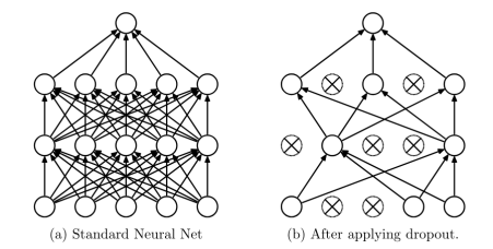
• Definition: Randomly selected neurons are temporarily deactivated during each iteration of training
  • Deactivated neurons output 0 during that training step, meaning they do not connect to the next layer
  • The dropout rate $p$ is set between 0 and 1, and determines the percentage of neurons to be randomly deactivated
  • This allows different sub-networks to be learned in each training step
  • Enhances the network’s generalization performance by preventing over-reliance on specific neurons

• Mathematical Representation

  • For the output $y$ of each neuron, a dropout mask $d$ is applied during training, which randomly deactivates certain neurons
  • Here, $d$ takes values between 0 and 1, with the probability of 0 determined by $p$
    $y_{\text{dropout}} = y \cdot d$
  • Where $d \sim Bernoulli(1-p)$, meaning $d$ becomes 0 with a probability of $p$ and 1 with a probability of $(1-p)$

• Dropout in Training vs. Inference

  • Training Phase
    • Neurons are either activated or deactivated according to the dropout rate
    • Neuron outputs are adjusted based on the dropout rate to prevent weight dependency on specific neurons
  • Inference Phase
    • Dropout is not applied; all neurons deactivated during training are reactivated to use the entire network
    • Instead, the output is adjusted based on the dropout rate
    • For example, with a dropout rate of 0.5 during training, each neuron output is divided by 0.5 during inference, creating a probabilistic ensemble effect to improve generalization
    • Therefore, the neuron output during inference is adjusted as follows:
      $y_{\text{inference}} = y \times (1 - p)$

🥨 Early Stopping

A technique to prevent overfitting by stopping training early when overfitting is detected

• Definition: Measures validation loss or validation accuracy periodically during training and stops training if no further improvement is observed

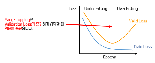
  • Typically, training loss decreases continuously, but at a certain point validation loss begins to increase. This indicates the model is overfitting to the training data, and Early Stopping halts training at this point.

    

• Early Stopping Implementation

  • Patience
    • Stops training if validation performance does not improve for a specified number of epochs
    • For example, with a patience of 5, training stops if validation performance does not improve for 5 consecutive epochs, allowing training to continue if performance fluctuates slightly without halting too early
  • Restore Best Weights
    • Restores model weights from the epoch with the best validation performance before halting
    • For instance, restores weights from the epoch with the lowest validation loss to save the model in its optimal state

• Mathematical Representation

  • Let $t$ denote the epoch at which validation loss is minimized:
    $t^* = \arg \min_t L_{\text{validation}}(t)$
    • $t^*$: The optimal epoch where Early Stopping halts training