Optimizer

💡 Optimizer

An algorithm to minimize the Loss Function

---

🥨 Gradient Descent

• Definition: A method to find the minimum value of a given function (usually a Cost function or Loss function) using its gradient.

  • When a function $f(x)$ is given, the goal is to find its minimum value -> Gradient Descent calculates the gradient $\Delta f(x)$ and moves in the opposite direction of the gradient.

• Formula

  $\theta = \theta - \eta\frac{\partial L}{\partial \theta}$
  • In the formula, $\eta$ is called the learning rate, which determines how much the parameters should be updated in one iteration, i.e., how much to adjust the parameter value.
  • This formula represents one iteration of the update, and in practice, this step is repeated multiple times.

• Example

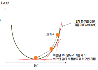
  • If the loss function is a parabolic second-order function like the figure below, Gradient Descent applies differentiation from the initial $\theta$, and then sequentially updates $\theta$ in the direction where the gradient of the function decreases.
  • Finally, it returns the value of $\theta$ at the point where the gradient no longer decreases, which is considered the point where the loss function is minimized.

  

🥨 Stochastic Gradient Descent

• Definition: Unlike standard Gradient Descent, which calculates the gradient over the entire dataset and updates the weights at once, SGD calculates the gradient for a single data point at a time and updates the weights immediately.

• SGD Update Formula

  $\mathbf{W} = \mathbf{W} - \eta \nabla L(\mathbf{W}; x^{(i)}, y^{(i)})$
  • $\theta$: The parameter to be learned.
  • $\eta$: Learning rate, which determines how much the parameter moves during one update.
  • $\Delta_\theta J (\theta;x^{(i)}, y^{(i)})$: The gradient of the cost function for the $i$-th data point $(x^{(i)}, y^{(i)})$.

• Operation Process

  1. Initialization: Randomly initialize the model's weight $\mathbf{W}$.
  2. Random Sample Selection: Randomly select one sample $(x^{(i)}, y^{(i)})$ from the dataset.
  3. Gradient Calculation: Calculate the gradient of the loss function $\nabla L(\mathbf{W}; x^{(i)}, y^{(i)})$ for that sample.
  4. Weight Update: Use the gradient to update the weight $\mathbf{W}$.
  5. Repeat: Repeat this process until all samples in the dataset are processed, and the training is performed over multiple epochs.

• Disadvantages

  • Oscillation and Instability: Since the gradient is calculated for random samples, the weight updates can be inconsistent and oscillate, which may slow down convergence.
  • Difficulty in Ensuring Convergence: Unlike standard Gradient Descent, the convergence of the loss function is not always guaranteed and can be unstable, so proper adjustment of the learning rate is crucial.

🥨 Mini-Batch Gradient Descent

• Definition: A method that divides the entire dataset into small batches and calculates the gradient for each mini-batch to update the weights.

  • Each mini-batch is composed of randomly selected samples from the entire dataset.
  • The gradient of the loss function is calculated using this mini-batch, and the weights are updated.

• Mini-Batch Gradient Descent Update Formula

  $\mathbf{W} = \mathbf{W} - \eta \frac{1}{|B|} \sum_{i \in B} \nabla L(\mathbf{W}; x^{(i)}, y^{(i)})$
  • $\mathbf{W}$: Weight vector of the model.
  • $\eta$: Learning rate.
  • $B$: A set of data samples in the mini-batch.
  • $|B|$: Size of the mini-batch.
  • $\nabla L(\mathbf{W}; x^{(i)}, y^{(i)})$: Gradient of the loss function for the sample $(x^{(i)}, y^{(i)})$.

• Operation Process

  1. Initialization: Randomly initialize the model's weights $\mathbf{W}$.
  2. Dataset Division: Divide the entire dataset into small mini-batches, each mini-batch consisting of $|B|$ data points.
  3. Mini-Batch Selection: Select one mini-batch $B$ and calculate the gradient.
  4. Gradient Calculation: Calculate the gradient of the loss function for all data points in the mini-batch and compute the average of the gradients.
  5. Weight Update: Update the weights using the average gradient from the mini-batch (using the formula above).
  6. Repeat: Repeat this process until all mini-batches in the dataset have been processed, and training is performed over multiple epochs.

• Disadvantages

  • Noise Issues: If the mini-batch size is too small, the gradient may oscillate like in SGD, causing slower or unstable convergence.
  • Impact of Mini-Batch Size: If the mini-batch size is too large, it may use too much memory and slow down learning like Batch Gradient Descent. If too small, it may cause noisy and unstable learning.
  • Computational Complexity: If hyperparameters are not set correctly, the learning process can be unstable or inefficient.

🥨 Momentum

• Definition: Instead of simply moving in the direction of the gradient, Momentum adds acceleration by partially reflecting the gradient information from the previous step.

  • It increases speed in flat regions and reduces oscillation in regions where the gradient changes sharply.

• Momentum Update Formula: The previous step's update is treated as an acceleration.

  • Velocity calculation:

    $v_t = \gamma v_{t-1} + \eta \nabla L(\mathbf{W})$

  • Weight update:

    $\mathbf{W} = \mathbf{W} - v_t$
    • $v_t$: Velocity, representing the direction of weight update.
    • $\gamma$: Momentum coefficient, determining how much of the previous gradient is reflected.
    • $\eta$: Learning rate.

• Features of Momentum

  • When Gradient Descent reaches flat regions of the loss function, the gradient becomes small, and weight updates slow down. Momentum maintains speed in such cases, enabling faster convergence by using the previous gradient.
  • Proper setting of the momentum coefficient $\gamma$ and learning rate $\eta$ is crucial.

🥨 RMSprop

• Definition: RMSprop calculates the moving average of the squared gradients and adjusts the learning rate based on the magnitude of the gradients.

  • It makes the size of each weight update inversely proportional to the size of the gradient.
  • Helps maintain a stable learning rate when the gradient magnitude varies significantly during training, particularly effective in mitigating the vanishing gradient problem.

• RMSprop Update Formula: The exponential moving average (EMA) of the squared gradient $g_t$ is calculated, and this is used to adjust the learning rate.

  • EMA of squared gradients calculation:

    $E[g^2]_t = \beta E[g^2]_{t-1} + (1 - \beta) g_t^2$
    • $E[g^2]_t$: Exponential moving average of the squared gradient at time step $t$
    • $g_t$: The current gradient
    • $\beta$: The decay rate of the exponential moving average, typically set to 0.9

  • Weight update:

    $\mathbf{W}_{t+1} = \mathbf{W}_t - \frac{\eta}{\sqrt{E[g^2]_t + \epsilon}} g_t$
    • $\eta$: Learning rate
    • $\epsilon$: A small constant for numerical stability, usually set to $10^{-8}$ to prevent division by zero
    • $g_t$: The current gradient

  • As shown in the formula, the larger the gradient, the smaller the learning rate becomes, and the smaller the gradient, the larger the learning rate. RMSprop dynamically adjusts the learning rate to perform appropriate weight updates.

• Disadvantages:

  • Complex Hyperparameter Tuning: Proper tuning of $\beta$ and $\eta$ is crucial.
  • Difficulty in Moving Toward Global Minimum: If it converges too quickly at the start of training, there is a risk of getting stuck in a local minimum.

    

🥨 Adam

• Definition: Adam is a combination of Momentum and RMSprop.

  • Adam uses separate learning rates for each weight and adaptively adjusts them while applying momentum to account for the direction of the gradients.
  • Adam updates the weights using two EMA estimates:
    • First Moment: The mean of the gradients, capturing the direction of the gradients through momentum.
    • Second Moment: The squared gradients, adjusting the learning rate based on gradient magnitude, similar to RMSprop.

• Adam Update Process:

  1. First Moment Estimate:
     The EMA of the gradient $g_t$ (first moment) is calculated as:

     $m_t = \beta_1 m_{t-1} + (1 - \beta_1) g_t$
     • $m_t$: Exponential moving average of the first moment (mean) of the gradient $g_t$
     • $\beta_1$: Decay rate for the first moment, typically set to 0.9
     • $g_t$: The current gradient

  2. Second Moment Estimate:
     The EMA of the squared gradient (second moment) $v_t$ is calculated as:

     $v_t = \beta_2 v_{t-1} + (1 - \beta_2) g_t^2$
     • $v_t$: Exponential moving average of the second moment (variance) of the squared gradient
     • $\beta_2$: Decay rate for the second moment, typically set to 0.999
     • $g_t^2$: The square of the current gradient

  3. Bias-Correction: At the early stages of Adam, the estimates for $m_t$ and $v_t$ are biased toward 0, so bias correction is applied:

     • Bias correction for the first moment:

       $\hat{m}_t = \frac{m_t}{1 - \beta_1^t}$

     • Bias correction for the second moment:

       $\hat{v}_t = \frac{v_t}{1 - \beta_2^t}$

  4. Weight Update: The weights are updated using the bias-corrected moment estimates:

     $\mathbf{W}_{t+1} = \mathbf{W}_t - \frac{\eta}{\sqrt{\hat{v}_t} + \epsilon} \hat{m}_t$
     • $\mathbf{W}_t$: The current weight
     • $\eta$: Learning rate
     • $\epsilon$: A small constant for numerical stability, typically set to $10^{-8}$ to prevent division by zero
     • $\hat{m}_t$: Bias-corrected first moment (mean of the gradients)
     • $\hat{v}_t$: Bias-corrected second moment (variance of the gradients)