ImageNet Classification with Deep Convolutional Neural Networks

ImageNet Classification with Deep Convolutional Neural Networks

---

Alex Krizhevsky / Ilya Sutskever/ Geoffrey E. Hinton.

Notice :

Since I have no interest in actual numbers or expressions , I’ll be skipping details of results

The purpose of this is for me to understand more about the concept of neural networks and learn how AI technology has been developing so far

Abstract

• a large deep convolutional neural network is trained to classify the 1.2 million high-resolution images in the ImageNet LSVRC-2010 contest into the 1000 different classes
• it achieved top1 and top5 error rates of 37.5% and 17%
• The neural network consists of five convolutional layers, and three fully-connected layers
• to make training faster, non-saturating neurons and very efficient GPU implemantation was used
• to reduce overfitting, ‘drop out’ as the regularization method in the fully-connected layers

Introduction

• until recently datasets were relatively small and recognition task can be solved quite well (error rate on MNIST digit-recognition task approaches human performance
• it has only recently become possible to collect labeled datasets with millions of images(LabelMe,ImageNet)
• to learn from larger datasets, need a large learning capacity. but the model also should have lots of prior knowledge to compensate for all the data we don’t have for immense complexity of the object recognition ( this problem cannot be specified by large dataset)
• Convolutional neural networks(CNNs)
  • their capacity can be controlled by varying their depth and breadth.
  • they also make strong and mostly correct assumptions about the natural images
  • they have much fewer connections and parameters which means they are easier to train
• Despite the attractive qualities and relative efficiency of their local architecture, it’s still been expensive to apply in large scale to high-resolution images → but the GPUs are powerful enough, and recent datasets contain enough labeled examples

The Dataset

• ImageNet is a dataset of over 15 million labeled high-resolution images belonging to roughly 22,000 categories
• there are roughly 1.2million training images, 50000 validation images, and 150000 testing images
• usually in ImageNet report two error rates : top1 and top5
• imagenet consist of variable-resolution images, still need to be dimensionally fixed to put in system
• did not pre-processed the images in any other way after down-sampling to fixed resolution of 256*256 except subtracting the mean activity over the training set from each pixel
• trained our network on the raw RGB values of the pixel

  what is error rate top1 and top 5 ?

The Architecture

• the architecture contains 8 learned layers
  • five convolutional layers
  • three fully-connected layers

ReLu Nonlinearity

• these saturating nonlinearities are much slower than the non-saturating nonlinearity f=max(0,x)
• we refer to neurons with this non-linearity as Rectified Linear Units
• train with ReLu is several times faster than their equivalents with tanh units
• this plot shows that we would not have been able to experiment with such large neural networks for this work if we had used traditional saturating neuron models

Training on multiple GPUs

• Because the GPU limits the maximum size of the networks that can be trained on it, we separated the net across two GPUs.
• current GPUs are partially well-suited to cross-GPU parallelization
• puts half of the kernels on each GPU and the GPU communicated only in certain layers → this allows to precisely tune the amount of communication

Local Response Normalization

• ReLu does not need to be normalized. However, if the weight of a specific pixel is high, the affected feature map may have a high number.
• This normalization was applied after the ReLu non-linearity in certain layers
• This sort of response normalization implements a form of lateral inhibition, creating competition for big activities amongst neuron outputs computed using different kernels

Overlapping pooling

• Pooling layers in CNNs summarize the outputs of neighboring groups of neurons in the same kernel map
• a pooling layer can be thought of as consisting of a grid of pooling units spaced s pixel apart, each summarizing a neighborhood of size z*z centered at the location of the pooling unit
  • s = z : traditional local pooling as commonly employed in CNNs
  • s < z : overlapping pooling

• this scheme reduces the top1 and top5 error rates compared to non-overlapping scheme
• the models with overlapping pooling slightly more difficult to overfit

Overall Architecture

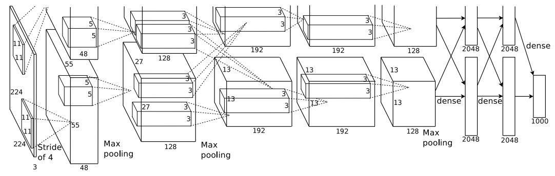
• five convolutional and the three fully-connected layers
• maximizes the multinomial logistic regression : maximizing the average accross the training cases of the log-probability of the correct label under the prdiction distribution
• second,fourth,fifth convolutional layers are connected only to those kernel maps in the previous layer which reside on the same GPU
• third convolutional layer are connected to all kernel maps in second layer
• the ReLu non-linearity is applied to the output of every convolutional and fully connected layer

Reducing Overfitting

Data Augmentation

• the easiest common method to reduce overfitting on image data is artificially enlarge the dataset using label-preserving transformations
• employed two distinct forms of data augmentation that allow transformed images to be produced from the original images with very little computation
  • generating image translations and horizontal reflections
    • to do this : extracting random patches and their horizontal reflections
    • train out network on these extracted patches
    • this increases the size of our training set ,highly interdependent
    • at test time, the network make prediction by extracting patches and reflections
    • and averaging the predictions made by softmax layer
  • altering the intensities of the RGB channels in training images
    • performed PCA on the set of RGB pixel values throughout the ImageNet training set

Dropout

• a very efficient version of model combination that only cost about a factor of two during training
• dropout consist of setting to zero the output of each hidden neuron with probability 0.5
• the neurons which are “dropped out” in this way do not contribute to the forward pass and do not participate in back-propagation
• this technique reduces complex co-adaptations of neurons
• force to learn more robust features that are useful in conjunction with many differnt random subsets of the other neurons
• dropout used in the first two fully-connected layers
• dropout roughly doubles the number of iterations required to converge

Details of learning

• stochastic gradient descent was used with batch size of 128 examples, momentum of 0.9, and weight decay 0.0005
• this small amount of weight decay was important to reduces the model’s training error
• initialized weights the weights to 0.01 , neuron biases in the second, fourth, fifth convolutional layers and fully-connected layers to 1
• used equal learning rate for all layers
  
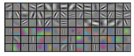
• this figure shows convolutional kernels.
  GPU 1 classifies images by oriented edge, and GPU 2 classifies images by color.

Results

• Through learning, kernels that are each color-bound and color-independent were created.
• Image classification in the hidden layer may be a much better method than conventional image search methods.

Discussion

• a large, deep convolutional neural network was able to achieve record-breaking results on a highly challenging dataset using purely supervised learning
• depth was really important to achieve this results