Variational transformer-based anomaly detection approach for multivariate time series
Paper Review
1. Introduction
Traditional Limitation
- Need to rely on expert experience to build complex feature
Previous Study & Necessity of this study
- Multivariate time-series data has potential correlation between time series
- It must be considered
- GNN extracts the potential correlation by constructing a feature relationship graph
- However, such algorithms depends too much on the size of the feature relationship graph
- When the grpah is too sparse or the number of feature nodes is too small, it cause the performance bottleneck of the model
→ We propose Transformer-based model to capture the correlation through the self-attention mechanism
- Why? → It reduces impact of the dimensionality of data
Main contributions
- Global temporal encoding (positional encoding)
- Multi-scale feature fusion algorithm
- Obtain robust feature expression
- Residual Variational AutoEncoder
- Can alleviate the KLD vanishing problem
2. Related work
2.1 Multivariate time-series anomaly detection
Challenging points
- Occurs with a periodic or seasonal mode
- Complex correlations between their sequences
We use self-attention mechanism to capture the corelation in feature dimensions
2.3 Variational AutoEncoder
Limitation of AutoEncoder for anomaly detection
- AE is only trained with as little reconstruction loss as possible, regardless of how the hidden space encoded
- In my opinion, Loss term of AE is only composed of Reconstruction loss
- It causes possibility of overfitting = lack of regularity in the hidden space
VAE
- forms robust local features
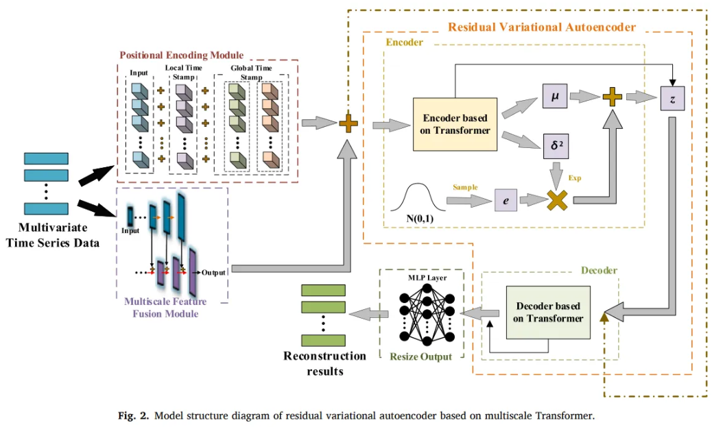
3. Multiscale transformer-based residual VAE
Limitation of traditional Transformer
- Only extract the local sequential information
- Cannot extract the global time-series information
- In the process of upsampling,
- Mapping relationship with raw input and high-dimensional vector (input data) is not accurate
Explanation of difference between the local and global information
For example, a traditional transformer model might effectively capture that a stock has been increasing for the last few days (local sequential information),
but it may not as easily recognize that the stock is in a long-term downward trend (global information), which is more complex and requires analyzing data over a longer period.
Model Parts
1. Positional encoding module
- Provide the model local sequential and global time-series information
2. Multi-scale feature fusion module
- Obtain more robust feature expression
3. Feature-learning module
- Learn both temporal and feature dimensions
- through Transformer and VAE
4. Data reconstruction module
- Conv1d layer and FC layer
3.1 Positional encoding
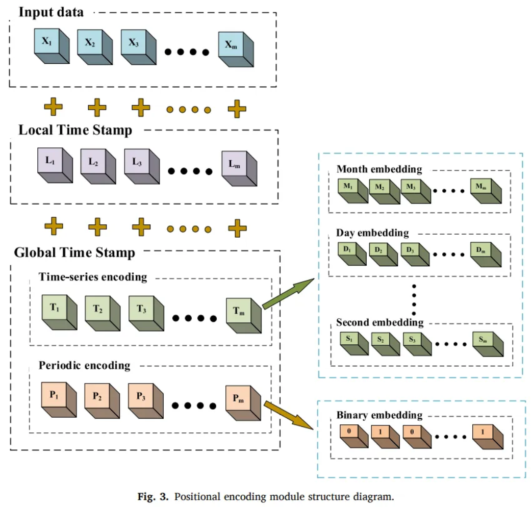
Global temporal encoding
-
Time-series encoding
- Decompose the time stamp information
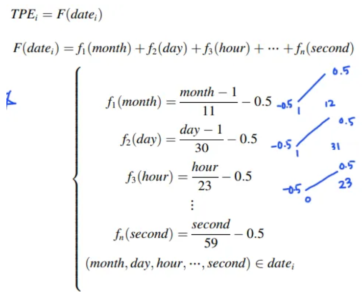
- Decompose the time stamp information
-
Periodic encoding
-
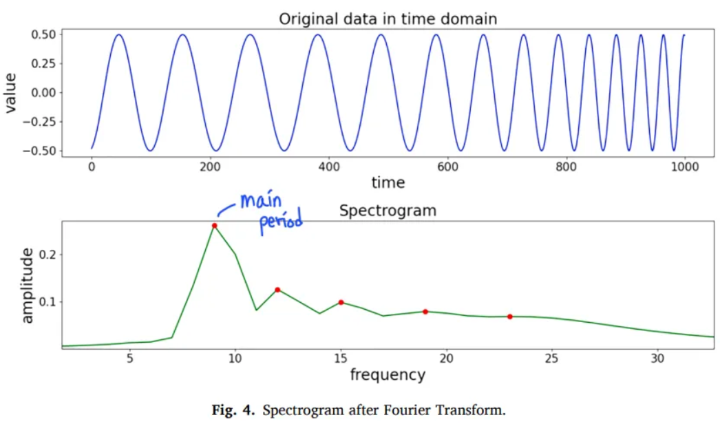
Fourier transform to analyze the period of time series data from frequency domain
-
The main period = The most significant impact on the time-series data
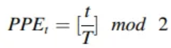
- T : the period of the data
- t : the timestamp
-
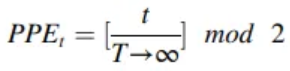
If time series data has no pattern or close to a constant value,
-
After Fourier transform, it’s a group of sine waves with tiny amplitude
-
Then, DC component is the most influential to the time series data
-
DC is a sine wave with an infinite period
-
Frequency → 0
-
Main period of the time series data →
-
Do not add extra information to non-periodic time series data
-
3.2 Multiscale feature fusion
- FC layer or Conv1d layer map input into a high-dimensional vector
- FC or Conv1d alone is not accurate
- Feature pyramid structure
- only handle image data
- Only convolves and up-samples in the time dimension
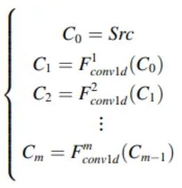
- : input data
- : number of conv layers
- Hyper parameter
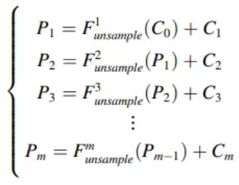
- : Transposed conv1d
- learnable parameters
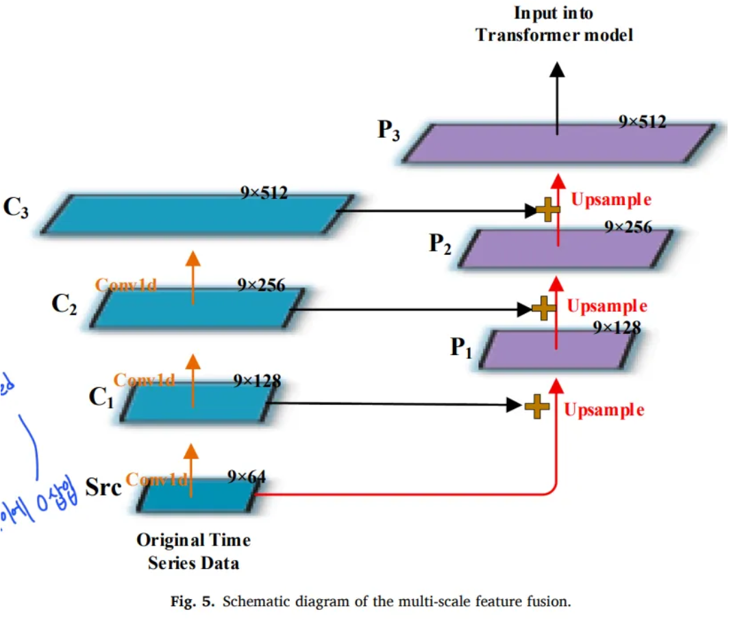
- interpolation need parameters and it’s not optimal
- Conv stride must be diveded into the size of the transposed conv kernel
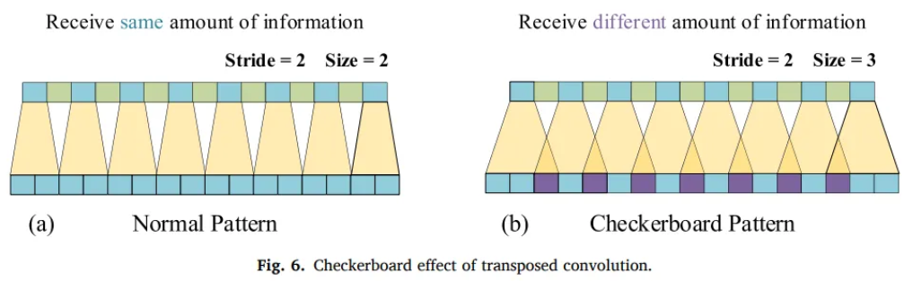
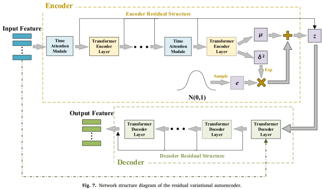
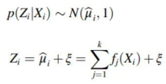
3.3 Residual Variational AutoEncoder
Loss term
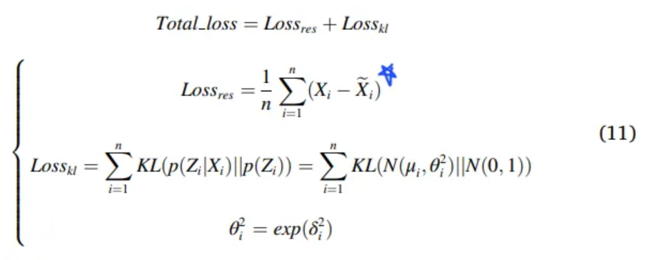
- and
- learnable parameter
- control value range of the variance to
- Prevent loss appearing negative
Reconstruction
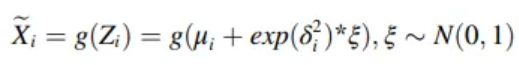
-
: Decoder function
-
: Noise sampled from the Standard normal distribution
-
When decoder is too powerful or the weight of the is too high,
-
model encodes all the input data into a Standard normal distribution
-
in order to obtain the minimum of the loss function
-
As a result, decoder only relies on the noise data
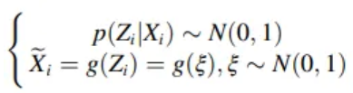
- KL divergence vanishing problem
- degenerate to the Standard normal distribution
- KL divergence vanishing problem
-
Transformer’s decoder is too powerful
→ Transformer-based VAE is more prone to disappearance of divergence
Traditional Solution
- Set dynamic coefficients for the term
- Long process of finding the suitable coefficient
- Reduce decoder’s performance, increasing the contribution of the reconstruction error term
- But, low performance decoder will reduce the model generation ability
Proposed Solution
- Residual VAE
- Do not connect the encoder and the decoder
- Combines the residuals separately
- Prevent encoder information from leaking to the decoder
- Add a time window-based attention to the encoder
Residual structure
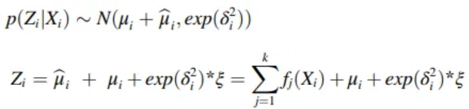
-
: constant term, output sum of the encoders of each layer
-
k : number of encoder layers
-
When the disappearance of divergence occurs = mean, var equals to 0
- Prevent degenarting to Standard normal distribution
- → Prevent the decoder from only reconstructing from the noise data
Time dimension attention mechanism
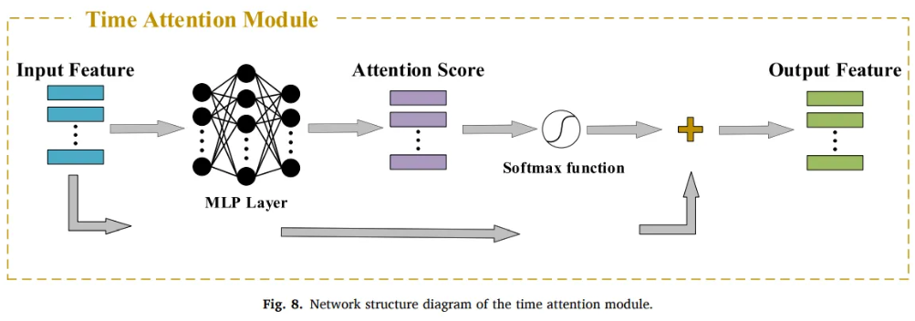
- Transformer-based model only capture feature dimension with self-attention
- Does not consider autocorrelation of data features in the time dimension
- Data at different moments have different effects on the data at the current moment
- Add weight information to the data in the same time window

- : a feature of input data in a time window
- l : width of the time window
- To prevent disappearance of divergence, only add to the encoder
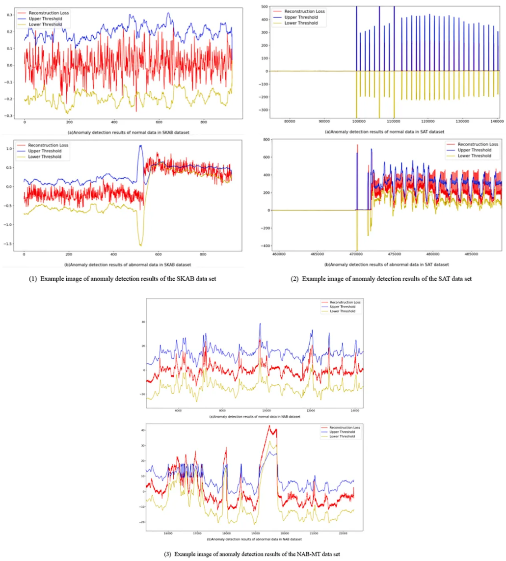
3.4 Data reconstruction and anomaly detection
- Conv1D and FC layer to adjust the output size
- Upper threshold limit based on the reconstruction loss under normal data
- Due to the changeable operating environment, difficult to apply the same upper threshold
Dynamic threshold method
- Record the reconstruction error at each moment as vector
- h : total time of detection data
- In order to reduce the influence caused by the normal fluctuation of the data,
- Use the exponentially weighted moving average algorithm EWMA to smooth
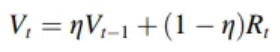
- : smoothed reconstruction error
- : actual reconstruction error at the current time
- : weight coefficient
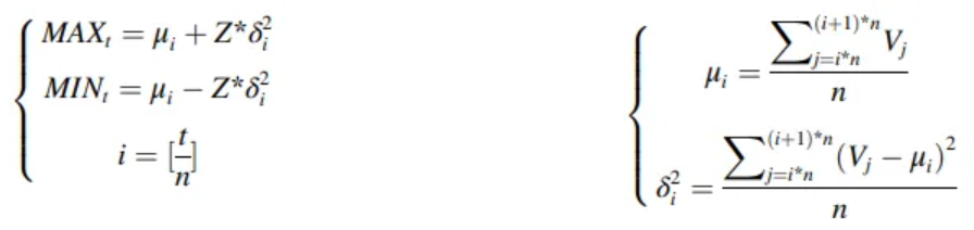
- Z : hyper parameter
- n : size of sliding window
- : mean value of the error vector V in the sliding window group i
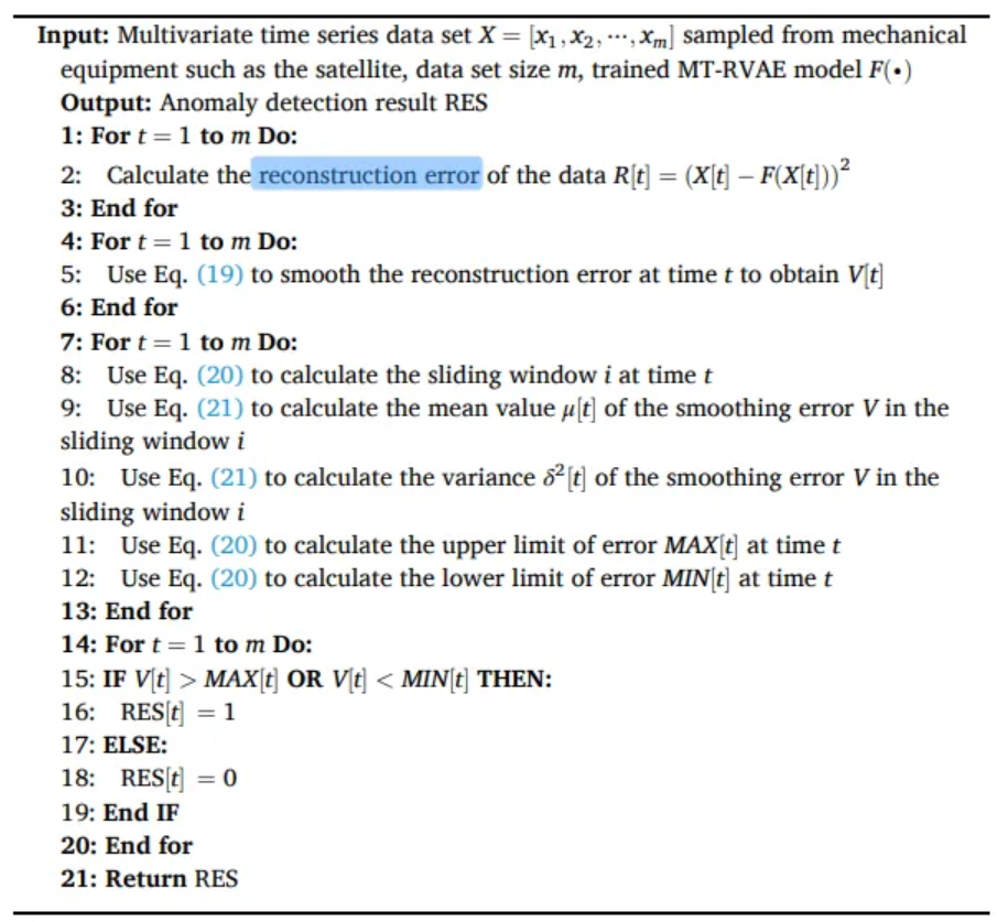
Algorithm steps
- Use the trained model to reconstruct the data and calculate the reconstruction error
- Use the EWMA to smooth the reconstruction error vector
- Calculate the error threshold at each moment
- Judge whether the point is an abnormal or normal
4. Experiments
4.1 Dataset
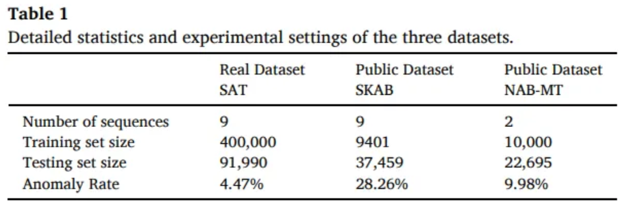
SKAB
- IIoT data
SAT
- satellite data
4.2 Baseline methods and model setting
Local outlier factor
Isolation forest
LSTM AE
Fault prediction based on LSTM
SOTA models
| GDN | Multivariate | Graph based |
|---|---|---|
| MTAD-GAT | Multivariate | Graph attention |
| LSCP | Parallel integration | |
| OmniAnomaly | VAE and GRU | |
| CPA-TCN | Temporal CNN | |
| TCN-AE | Temporal CNN and AE |
- Debug the parameters of the above methods to obtain the best results
Model parameter
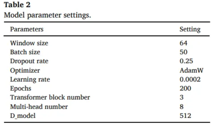
4.3 Comparison
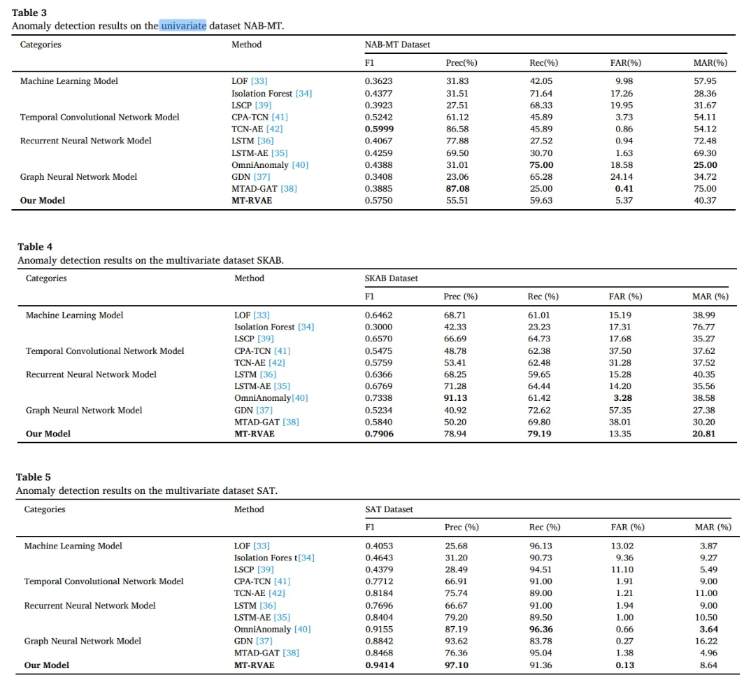
- ML algorithms that cannot capture temporal dependency perform poorly in NAB-MT
- MT-RVAE and GNN which focus on the multidimension is not as good as the TCN-AE on the one-dimensional data
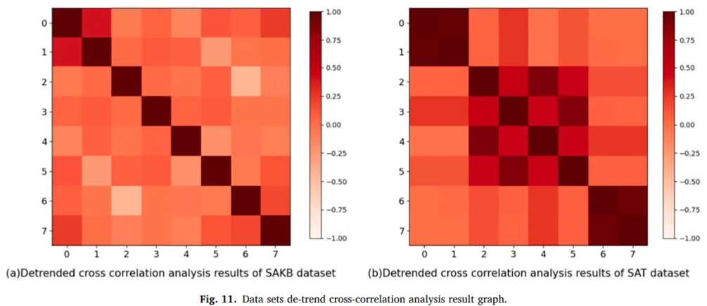
-
Relationship between the different attributes of SKAB is sparse
-
Real dataset SAT has more relationship between the attributes
-
→ Performance of GNN model on the SAT is higher
-
However, SAT has only 9 dimensions, the upper limit is low, which causes a bottleneck in GNN
-
OmniAnomaly (VAE + GRU) does not consider correlation between sequences
-
→ Lower than MT-RVAE
-
MT-RVAE can capture the correlation between different sequences through self attention
-
→ Don’t need to extract information through the feature relationship graph
-
→ Avoid the information bottleneck caused by node sparseness
-
Global temporal encoding and residual VAE can extract the temporal dependence and local features
Conclusions
-
Model rely only on the temporal dependence in the data, will not improve the accuracy for multivariate time series
-
Performance on the GNN in SAT is higher than RNN and TCN, which proves the importance of capturing the sequence correlation
-
Tightness of data feature relationship will affect the performance of GNN algorithm
-
OmniAnomaly algorithm proves the number of features of the data will cause the bottleneck
-
MT-RVAE can effectively capture the temporal dependence and sequence correlation
-
Unidimensional or have no correlation between sequences are more suitable on TCN or RNN
-
Multidimensional or have the correlation between sequences are more suitable on GNN or Transformer
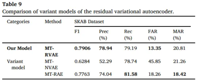
4.4 Ablation Study
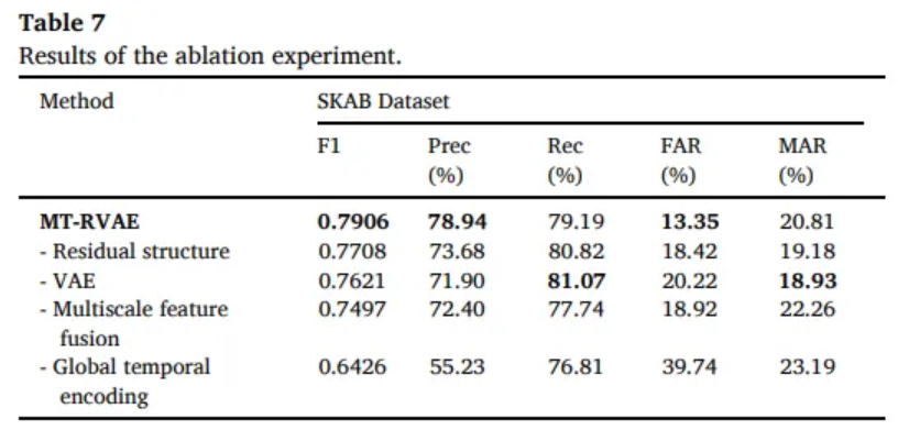
- Residual structure can alleviate the disappearance of the divergence
- Hidden space encoded by VAE can improve the performance
- Multi-scale feature can help the model better distinguish abnormal point
- Global temporal encoding capture the long time dependencies
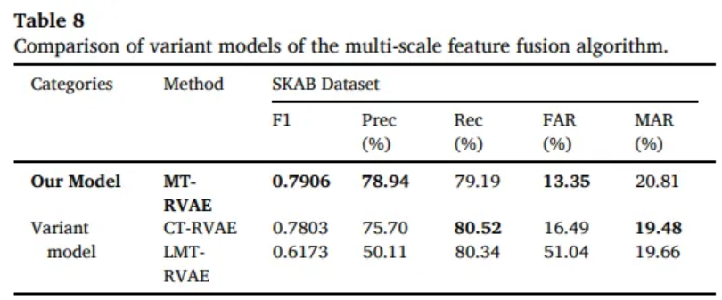
CT-RVAE
- Conv1D instead of Multi-scale feature fusion
LMT-RVAE
- Bilinear interpolation instead of Transposed convolution for upsampling
MT-NVAE
- Ordinary residual structure instead of residual
MT-RAE
- Residual AE instead of RVAE