인구 데이터 기반 소득 예측
- 본 포스팅은 데이콘의
인구 데이터 기반 소득 예측 경진대회에 참여하여 작성한 코드이며, 간단한 데이터 전처리 및 EDA, LightGBM과 XGBoost로 Ensemble 모델링 등의 내용을 포함하고 있습니다. - 코드실행은 Google Colab의 GPU, Standard RAM 환경에서 진행했습니다.
- Keyword : 소득예측, classification, lightgbm, xgboost, ensemble, voting
➔ 데이콘에서 읽기 - 👉
Click
0. Import Packages
from google.colab import drive
drive.mount('/content/drive')
Mounted at /content/drive
!pip install -U pandas-profilingimport numpy as np
import pandas as pd
import matplotlib
import matplotlib.pyplot as plt
import sklearn
import pandas_profiling
import seaborn as sns
import random as rn
import os
import scipy.stats as stats
from sklearn.preprocessing import LabelEncoder
from sklearn.preprocessing import OneHotEncoder
from sklearn.model_selection import train_test_split
from sklearn.ensemble import VotingClassifier
from sklearn import metrics
import xgboost as xgb
import lightgbm as lgb
from collections import Counter
import warnings
%matplotlib inline
warnings.filterwarnings(action='ignore')print("numpy version: {}". format(np.__version__))
print("pandas version: {}". format(pd.__version__))
print("matplotlib version: {}". format(matplotlib.__version__))
print("scikit-learn version: {}". format(sklearn.__version__))
print("xgboost version: {}". format(xgb.__version__))
print("lightgbm version: {}". format(lgb.__version__))numpy version: 1.21.6 pandas version: 1.3.5 matplotlib version: 3.2.2 scikit-learn version: 1.0.2 xgboost version: 0.90 lightgbm version: 2.2.3
# reproducibility
seed_num = 42   ####
np.random.seed(seed_num)
rn.seed(seed_num)
os.environ['PYTHONHASHSEED']=str(seed_num)
1. Load and Check Dataset
Variable Description
|age|workclass|fnlwgt|education|education.num|marital.status|occupation|
|나이|일 유형|CPS(Current Population Survey) 가중치|교육수준|교육수준 번호|결혼 상태|직업|
|relationship|race|sex|capital.gain|capital.loss|hours.per.week|native.country|
|가족관계|인종|성별|자본 이익|자본 손실|주당 근무시간|본 국적|
train = pd.read_csv('/content/drive/MyDrive/Forecasting_income/dataset/train.csv')
test = pd.read_csv('/content/drive/MyDrive/Forecasting_income/dataset/test.csv')

train.columns = train.columns.str.replace('.','_')
test.columns = test.columns.str.replace('.','_')

train.head()
id age workclass fnlwgt education education_num marital_status \
0 0 32 Private 309513 Assoc-acdm 12 Married-civ-spouse
1 1 33 Private 205469 Some-college 10 Married-civ-spouse
2 2 46 Private 149949 Some-college 10 Married-civ-spouse
3 3 23 Private 193090 Bachelors 13 Never-married
4 4 55 Private 60193 HS-grad 9 Divorced
occupation relationship race sex capital_gain capital_loss \
0 Craft-repair Husband White Male 0 0
1 Exec-managerial Husband White Male 0 0
2 Craft-repair Husband White Male 0 0
3 Adm-clerical Own-child White Female 0 0
4 Adm-clerical Not-in-family White Female 0 0
hours_per_week native_country target
0 40 United-States 0
1 40 United-States 1
2 40 United-States 0
3 30 United-States 0
4 40 United-States 0
pr=train.profile_report()
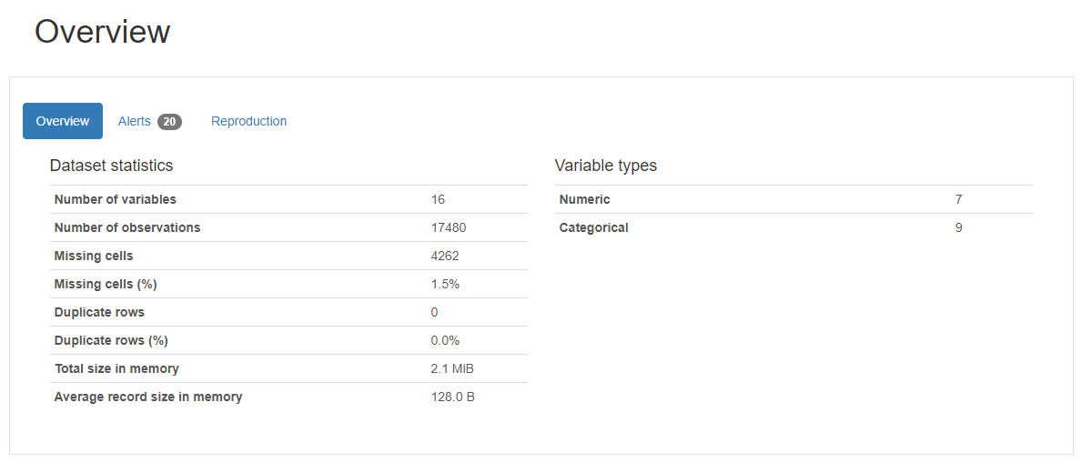
pr.to_file('/content/drive/MyDrive/Forecasting_income/pr_report.html')📝 Pandas profiling을 활용하면 아래와 같이 데이터 프레임을 쉽고 효율적으로 탐색할 수 있습니다.
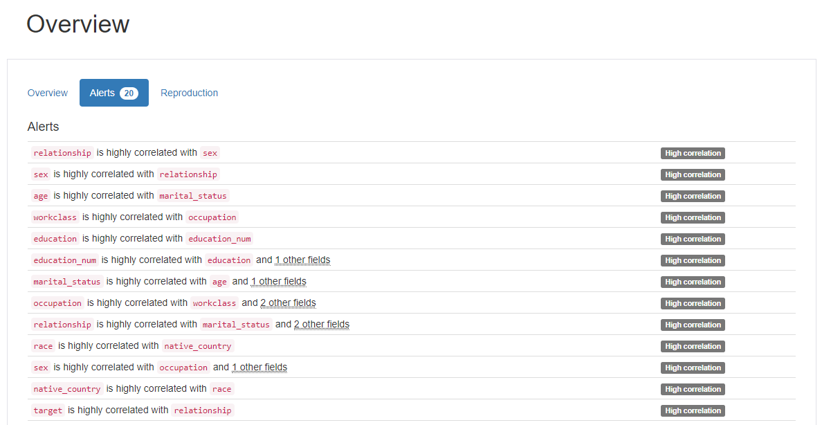
Pandas profiling report의 Alert 활용하기
High Correlation
-
relationship-sex -
age-marital.status -
workclass-occupation -
education-education.num -
relationship-marital.status -
race-native.country -
sex-occupation -
target-relationship
Data Type
-
Numeric (7) :
id,age,fnlwgt,education.num,capital.gain,capital.loss,hours.per.week -
Categorical (9) :
workclass,education,marital.status,occupation,relationship,race,sex,native.country,target
Note
📝 workclass와 occupation이 같은 비율 (10.5%)의 missing value를 가지므로 확인해 볼 필요가 있습니다.
📝 또한, native.country는 583(3.3%) missing value를 가지므로 행을 삭제해주겠습니다.
📝 capital.gain, capital.loss가 high skewness를 가집니다. outlier를 확인하고 필요시 transformation을 진행하겠습니다.
train.info()RangeIndex: 17480 entries, 0 to 17479 Data columns (total 16 columns): # Column Non-Null Count Dtype --- ------ -------------- ----- 0 id 17480 non-null int64 1 age 17480 non-null int64 2 workclass 15644 non-null object 3 fnlwgt 17480 non-null int64 4 education 17480 non-null object 5 education_num 17480 non-null int64 6 marital_status 17480 non-null object 7 occupation 15637 non-null object 8 relationship 17480 non-null object 9 race 17480 non-null object 10 sex 17480 non-null object 11 capital_gain 17480 non-null int64 12 capital_loss 17480 non-null int64 13 hours_per_week 17480 non-null int64 14 native_country 16897 non-null object 15 target 17480 non-null int64 dtypes: int64(8), object(8) memory usage: 2.1+ MB
2. Data Preprocessing
(1) Missing Value
train.columns[train.isnull().any()]Index(['workclass', 'occupation', 'native_country'], dtype='object')
train[train["workclass"].isnull()] id age workclass fnlwgt education education_num \
15081 15081 90 NaN 77053 HS-grad 9
15082 15082 66 NaN 186061 Some-college 10
15084 15084 51 NaN 172175 Doctorate 16
15086 15086 61 NaN 135285 HS-grad 9
15087 15087 71 NaN 100820 HS-grad 9
... ... ... ... ... ... ...
17475 17475 35 NaN 320084 Bachelors 13
17476 17476 30 NaN 33811 Bachelors 13
17477 17477 71 NaN 287372 Doctorate 16
17478 17478 41 NaN 202822 HS-grad 9
17479 17479 72 NaN 129912 HS-grad 9
marital_status occupation relationship race \
15081 Widowed NaN Not-in-family White
15082 Widowed NaN Unmarried Black
15084 Never-married NaN Not-in-family White
15086 Married-civ-spouse NaN Husband White
15087 Married-civ-spouse NaN Husband White
... ... ... ... ...
17475 Married-civ-spouse NaN Wife White
17476 Never-married NaN Not-in-family Asian-Pac-Islander
17477 Married-civ-spouse NaN Husband White
17478 Separated NaN Not-in-family Black
17479 Married-civ-spouse NaN Husband White
sex capital_gain capital_loss hours_per_week native_country \
15081 Female 0 4356 40 United-States
15082 Female 0 4356 40 United-States
15084 Male 0 2824 40 United-States
15086 Male 0 2603 32 United-States
15087 Male 0 2489 15 United-States
... ... ... ... ... ...
17475 Female 0 0 55 United-States
17476 Female 0 0 99 United-States
17477 Male 0 0 10 United-States
17478 Female 0 0 32 United-States
17479 Male 0 0 25 United-States
target
15081 0
15082 0
15084 1
15086 0
15087 0
... ...
17475 1
17476 0
17477 1
17478 0
17479 0
[1836 rows x 16 columns]
train['workclass'].unique()array(['Private', 'State-gov', 'Local-gov', 'Self-emp-not-inc',
'Self-emp-inc', 'Federal-gov', 'Without-pay', nan, 'Never-worked'],
dtype=object)
📝 workclass, occupation 컬럼의 결측치를 포함한 행은 삭제합니다.
📝 두 컬럼이 동시에 결측치를 갖는 경우가 대부분이었기에 workclass의 결측치만 'Never-worked'와 같은 이미 존재하는 특성으로 채우는것은 의미가 없습니다.
📝 workclass와 occupation에 새 feature을 생성하여 넣는 방법도 시도했지만, one-hot encoding을 해서 생기는 test 데이터와의 컬럼 차이 때문에 다른 방법을 고려해볼 필요가 있다고 생각합니다. 😔😔
print(sum(train['workclass'].isna()))
print(sum(train['occupation'].isna()))

fill_na = train['workclass'].isna()
1836 1843
df_train = train.dropna()

print(sum(df_train['workclass'].isna()))
print(sum(df_train['occupation'].isna()))
print(sum(df_train['native_country'].isna()))
0 0 0
df_train id age workclass fnlwgt education education_num \
0 0 32 Private 309513 Assoc-acdm 12
1 1 33 Private 205469 Some-college 10
2 2 46 Private 149949 Some-college 10
3 3 23 Private 193090 Bachelors 13
4 4 55 Private 60193 HS-grad 9
... ... ... ... ... ... ...
15076 15076 35 Private 337286 Masters 14
15077 15077 36 Private 182074 Some-college 10
15078 15078 50 Self-emp-inc 175070 Prof-school 15
15079 15079 39 Private 202937 Some-college 10
15080 15080 33 Private 96245 Assoc-acdm 12
marital_status occupation relationship race \
0 Married-civ-spouse Craft-repair Husband White
1 Married-civ-spouse Exec-managerial Husband White
2 Married-civ-spouse Craft-repair Husband White
3 Never-married Adm-clerical Own-child White
4 Divorced Adm-clerical Not-in-family White
... ... ... ... ...
15076 Never-married Exec-managerial Not-in-family Asian-Pac-Islander
15077 Divorced Adm-clerical Not-in-family White
15078 Married-civ-spouse Prof-specialty Husband White
15079 Divorced Tech-support Not-in-family White
15080 Married-civ-spouse Prof-specialty Husband White
sex capital_gain capital_loss hours_per_week native_country \
0 Male 0 0 40 United-States
1 Male 0 0 40 United-States
2 Male 0 0 40 United-States
3 Female 0 0 30 United-States
4 Female 0 0 40 United-States
... ... ... ... ... ...
15076 Male 0 0 40 United-States
15077 Male 0 0 45 United-States
15078 Male 0 0 45 United-States
15079 Female 0 0 40 Poland
15080 Male 0 0 50 United-States
target
0 0
1 1
2 0
3 0
4 0
... ...
15076 0
15077 0
15078 1
15079 0
15080 0
[15081 rows x 16 columns]
(2) Outlier
fig, ax = plt.subplots(1, 2, figsize=(12,3))
g = sns.distplot(df_train['capital_gain'], color='b', label='Skewness : {:.2f}'.format(df_train['capital_gain'].skew()), ax=ax[0])
g = g.legend(loc='best')

g = sns.distplot(df_train['capital_loss'], color='b', label='Skewness : {:.2f}'.format(df_train['capital_loss'].skew()), ax=ax[1])
g = g.legend(loc='best')
plt.show()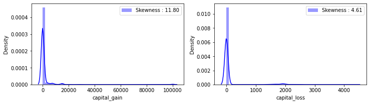
numeric_fts = ['age', 'fnlwgt', 'education_num', 'capital_gain', 'capital_loss', 'hours_per_week']

outlier_ind = []
for i in numeric_fts:
  Q1 = np.percentile(df_train[i],25)
  Q3 = np.percentile(df_train[i],75)
  IQR = Q3-Q1
  outlier_list = df_train[(df_train[i] < Q1 - IQR * 1.5) | (df_train[i] > Q3 + IQR * 1.5)].index
  outlier_ind.extend(outlier_list)
outlier_ind = Counter(outlier_ind)
multi_outliers = list(k for k,j in outlier_ind.items() if j > 2)# Drop outliers
train_df = df_train.drop(multi_outliers, axis = 0).reset_index(drop = True)
train_df id age workclass fnlwgt education education_num \
0 0 32 Private 309513 Assoc-acdm 12
1 1 33 Private 205469 Some-college 10
2 2 46 Private 149949 Some-college 10
3 3 23 Private 193090 Bachelors 13
4 4 55 Private 60193 HS-grad 9
... ... ... ... ... ... ...
15043 15076 35 Private 337286 Masters 14
15044 15077 36 Private 182074 Some-college 10
15045 15078 50 Self-emp-inc 175070 Prof-school 15
15046 15079 39 Private 202937 Some-college 10
15047 15080 33 Private 96245 Assoc-acdm 12
marital_status occupation relationship race \
0 Married-civ-spouse Craft-repair Husband White
1 Married-civ-spouse Exec-managerial Husband White
2 Married-civ-spouse Craft-repair Husband White
3 Never-married Adm-clerical Own-child White
4 Divorced Adm-clerical Not-in-family White
... ... ... ... ...
15043 Never-married Exec-managerial Not-in-family Asian-Pac-Islander
15044 Divorced Adm-clerical Not-in-family White
15045 Married-civ-spouse Prof-specialty Husband White
15046 Divorced Tech-support Not-in-family White
15047 Married-civ-spouse Prof-specialty Husband White
sex capital_gain capital_loss hours_per_week native_country \
0 Male 0 0 40 United-States
1 Male 0 0 40 United-States
2 Male 0 0 40 United-States
3 Female 0 0 30 United-States
4 Female 0 0 40 United-States
... ... ... ... ... ...
15043 Male 0 0 40 United-States
15044 Male 0 0 45 United-States
15045 Male 0 0 45 United-States
15046 Female 0 0 40 Poland
15047 Male 0 0 50 United-States
target
0 0
1 1
2 0
3 0
4 0
... ...
15043 0
15044 0
15045 1
15046 0
15047 0
[15048 rows x 16 columns]
print(train_df['capital_gain'].skew(), train_df['capital_loss'].skew())12.004940559585881 4.607122286739042
📝 Outlier들을 제거했음에도 두 변수는 여전히 high skewness를 가지고 있으므로 log transformation을 진행해보고자 합니다.
# log transformation
train_df['capital_gain'] = train_df['capital_gain'].map(lambda i: np.log(i) if i > 0 else 0)
test['capital_gain'] = test['capital_gain'].map(lambda i: np.log(i) if i > 0 else 0)

train_df['capital_loss'] = train_df['capital_loss'].map(lambda i: np.log(i) if i > 0 else 0)
test['capital_loss'] = test['capital_loss'].map(lambda i: np.log(i) if i > 0 else 0)print(train_df['capital_gain'].skew(), train_df['capital_loss'].skew())3.0945787119106676 4.390015583095806
3. Feature Engineering
(1) Correlation
📝 Categorical 데이터를 라벨인코더를 통해 수치형으로 변환한 후 상관관계를 확인합니다.
📝 Categorical : workclass, education, marital.status, occupation, relationship, race, sex, native.country
la_train = train_df.copy()

cat_fts = ['workclass', 'education', 'marital_status', 'occupation', 'relationship', 'race', 'sex', 'native_country']
for i in range(len(cat_fts)):
  encoder = LabelEncoder()
la_train[cat_fts[i]] = encoder.fit_transform(la_train[cat_fts[i]])la_train.head()id age workclass fnlwgt education education_num marital_status \ 0 0 32 2 309513 7 12 2 1 1 33 2 205469 15 10 2 2 2 46 2 149949 15 10 2 3 3 23 2 193090 9 13 4 4 4 55 2 60193 11 9 0 occupation relationship race sex capital_gain capital_loss \ 0 2 0 4 1 0.0 0.0 1 3 0 4 1 0.0 0.0 2 2 0 4 1 0.0 0.0 3 0 3 4 0 0.0 0.0 4 0 1 4 0 0.0 0.0 hours_per_week native_country target 0 40 38 0 1 40 38 1 2 40 38 0 3 30 38 0 4 40 38 0
📝 앞서 수행한 pandas profiling report의 alert를 참고하여 상관계수를 계산했습니다.
📝 꽤 유의미한 상관관계를 가지고 있다고 생각되는것은 relationship-sex, occupation-workclass, education-education.num 입니다.
# Pearson
la_train[['age','marital_status', 'relationship', 'sex', 'occupation', 'workclass']].corr()
age marital_status relationship sex occupation \
age 1.000000 -0.271955 -0.240331 0.087515 -0.007994
marital_status -0.271955 1.000000 0.180281 -0.124481 0.023856
relationship -0.240331 0.180281 1.000000 -0.590077 -0.052109
sex 0.087515 -0.124481 -0.590077 1.000000 0.061443
occupation -0.007994 0.023856 -0.052109 0.061443 1.000000
workclass 0.081100 -0.044000 -0.070512 0.078764 0.010194
workclass
age 0.081100
marital_status -0.044000
relationship -0.070512
sex 0.078764
occupation 0.010194
workclass 1.000000
la_train[['education', 'education_num', 'race', 'native_country']].corr()education education_num race native_country education 1.000000 0.348614 0.011236 0.079063 education_num 0.348614 1.000000 0.034686 0.097485 race 0.011236 0.034686 1.000000 0.126654 native_country 0.079063 0.097485 0.126654 1.000000
📝 Categorical 인 두 변수의 경우는 Cramer's V 공식을 활용하여 상관관계를 확인했습니다.
stat = stats.chi2_contingency(la_train[['race', 'native_country']].values, correction=False)[0]
obs = np.sum(la_train[['race', 'native_country']].values)
mini = min(la_train[['race', 'native_country']].values.shape)-1

# Cramer's V
V = np.sqrt((stat/(obs*mini)))
print(V)
0.11306993147326666
(2) String to numerical
📝 Categorical 데이터를 모델에 넣기 위해서는 수치화 시킬 필요가 있습니다. LabelEncoder는 불필요한 상관관계를 만들 가능성이 있기에 OnehotEncoder를 사용했습니다.
📝 Categorical : workclass, education, marital.status, occupation, relationship, race, sex, native.country
train_dataset = train_df.copy()
test_dataset = test.copy()
📝 get_dummies를 사용하여 one-hot encoding을 진행했습니다.
train_dataset = pd.get_dummies(train_dataset)
test_dataset = pd.get_dummies(test_dataset)

print(train_dataset.columns)
print(test_dataset.columns)
Index(['id', 'age', 'fnlwgt', 'education_num', 'capital_gain', 'capital_loss',
'hours_per_week', 'target', 'workclass_Federal-gov',
'workclass_Local-gov',
...
'native_country_Portugal', 'native_country_Puerto-Rico',
'native_country_Scotland', 'native_country_South',
'native_country_Taiwan', 'native_country_Thailand',
'native_country_Trinadad&Tobago', 'native_country_United-States',
'native_country_Vietnam', 'native_country_Yugoslavia'],
dtype='object', length=106)
Index(['id', 'age', 'fnlwgt', 'education_num', 'capital_gain', 'capital_loss',
'hours_per_week', 'workclass_Federal-gov', 'workclass_Local-gov',
'workclass_Private',
...
'native_country_Portugal', 'native_country_Puerto-Rico',
'native_country_Scotland', 'native_country_South',
'native_country_Taiwan', 'native_country_Thailand',
'native_country_Trinadad&Tobago', 'native_country_United-States',
'native_country_Vietnam', 'native_country_Yugoslavia'],
dtype='object', length=104)
📝 train과 test의 열길이를 맞춰주는 작업을 합니다.
test_col = []
add_test = []

for i in test_dataset.columns:
    test_col.append(i)
for j in train_dataset.columns:
    if j not in test_col:
        add_test.append(j)
add_test.remove('target')
📝 test 데이터의 native.country 컬럼에는 'Holand-Netherlands' 특성이 없는걸까요?
print(add_test)['native_country_Holand-Netherlands']
for d in add_test:
test_dataset[d] = 0print(train_dataset.columns)
print(test_dataset.columns)Index(['id', 'age', 'fnlwgt', 'education_num', 'capital_gain', 'capital_loss',
'hours_per_week', 'target', 'workclass_Federal-gov',
'workclass_Local-gov',
...
'native_country_Portugal', 'native_country_Puerto-Rico',
'native_country_Scotland', 'native_country_South',
'native_country_Taiwan', 'native_country_Thailand',
'native_country_Trinadad&Tobago', 'native_country_United-States',
'native_country_Vietnam', 'native_country_Yugoslavia'],
dtype='object', length=106)
Index(['id', 'age', 'fnlwgt', 'education_num', 'capital_gain', 'capital_loss',
'hours_per_week', 'workclass_Federal-gov', 'workclass_Local-gov',
'workclass_Private',
...
'native_country_Puerto-Rico', 'native_country_Scotland',
'native_country_South', 'native_country_Taiwan',
'native_country_Thailand', 'native_country_Trinadad&Tobago',
'native_country_United-States', 'native_country_Vietnam',
'native_country_Yugoslavia', 'native_country_Holand-Netherlands'],
dtype='object', length=105)
📝 Train의 target column을 제외하고 보면 열길이가 잘 맞춰진것을 확인할 수 있습니다.
4. Modeling
📝 먼저, train과 validation 데이터를 train_test_split 함수를 사용하여 나눠줍니다.
test_size =0.15

train_data, val_data = train_test_split(train_dataset, test_size = test_size, random_state = seed_num)

drop_col = ['target', 'id']

train_x = train_data.drop(drop_col, axis = 1)
train_y = pd.DataFrame(train_data['target'])

val_x = val_data.drop(drop_col, axis = 1)
val_y = pd.DataFrame(val_data['target'])print(train_x.shape, train_y.shape)
print(val_x.shape, val_y.shape)(12790, 104) (12790, 1) (2258, 104) (2258, 1)
📝 LGBM과 XGboost를 Soft Voting하여 간단한 ensemble 모델을 제작했습니다.
📝 Soft Voting은 LGBM, XGboost 모델의 예측 확률을 평균하여 최종 class를 결정합니다.
LGBClassifier = lgb.LGBMClassifier(random_state = seed_num)lgbm = LGBClassifier.fit(train_x.values,
train_y.values.ravel(),
eval_set = [(train_x.values, train_y), (val_x.values, val_y)],
eval_metric ='auc', early_stopping_rounds = 1000,
verbose = True)XGBClassifier = xgb.XGBClassifier(max_depth = 6, learning_rate = 0.01, n_estimators = 10000, random_state = seed_num)xgb = XGBClassifier.fit(train_x.values,
train_y.values.ravel(),
eval_set = [(train_x.values, train_y), (val_x.values, val_y)],
eval_metric = 'auc', early_stopping_rounds = 1000,
verbose = True)voting = VotingClassifier(estimators=[('xgb', xgb),('lgbm', lgbm)], voting='soft')
vot = voting.fit(train_x.values, train_y.values)5. Evaluation & Submission
l_val_y_pred = lgbm.predict(val_x.values)
x_val_y_pred = xgb.predict(val_x.values)
v_val_y_pred = vot.predict(val_x.values)print(metrics.accuracy_score(l_val_y_pred, val_y))
print(metrics.accuracy_score(x_val_y_pred, val_y))
print(metrics.accuracy_score(v_val_y_pred, val_y))0.8702391496899912 0.8680248007085917 0.8596102745792737
print(metrics.classification_report(v_val_y_pred, val_y)) precision recall f1-score support
0 0.93 0.89 0.91 1800
1 0.63 0.72 0.68 458
accuracy 0.86 2258
macro avg 0.78 0.81 0.79 2258
weighted avg 0.87 0.86 0.86 2258
val_xgb = pd.Series(l_val_y_pred, name="XGB")
val_lgbm = pd.Series(x_val_y_pred, name="LGBM")
ensemble_results = pd.concat([val_xgb,val_lgbm],axis=1)
sns.heatmap(ensemble_results.corr(), annot=True)
plt.show()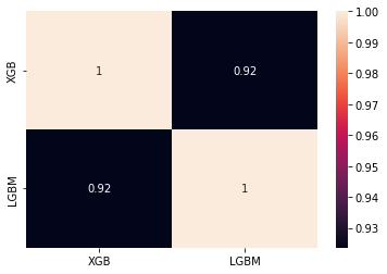
📝 Soft Voting을 진행했음에도 성능이 향상되지 않았습니다.
📝 두 모델의 예측은 높은 상관관계를 가지고 있었기에 앙상블 이전보다 성능이 향상되지 않았다고 해석할 수 있습니다.
(조금 더 공부가 필요할것 같습니다 😂😂)
감사합니다 :)
도움이 됐길 바랍니다👍👍