<References>
A Gentle Introduction to Graph Neural Networks
Graphs and where to find them
-
Images as graphs
224x224x3 floats → 1 pixel = 1 node
each nodes’ feature vector : 3-dimensional vector representing RGB value
non-border pixel은 8개의 이웃을 가지게됨 → adjacency matrix
-
Text as graphs
단어/토큰/문자(=node)의 연결 = directed graph
ex. Graphs are all around us ⇒ (Graphs) → (are) → (all) → (around) → (us)
하지만, image와 text의 encoding으로 graph를 잘 사용하지 않음
→ Since they have Regular structure!
-
Graph-valued data in the wild
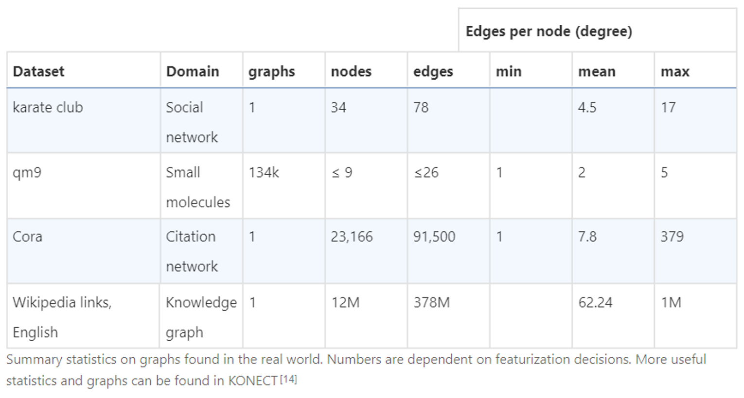
- Molecules as graphs
- Social networks as graphs
- Citation networks as graphs
- Other examples
What types of problems have graph structured data?
1. Graph-level task
Goal : predict the property of an entire graph
ex. Molecule의 구조가 주어졌을 때 해당 분자의 특성 알아내기
2. Node-level task
Goal : predict the identity or role of each node within a graph
ex. 네트워크 내의 노드 특성 분류
3. Edge-level task
Goal : predict the property of an entire graph
ex. 노드간의 연결 여부 예측, 연결 특성 분류
The challenges of using graphs in machine learning
4 Types of information on Graph : nodes, edges, global-context, connectivity
nodes, edges, global-context → 노드에 id를 부여하고 Matrix만들기
connectivity → Adjacency Matrix
👍) easily tensoriable
👎) 노드수가 많고 연결수가 적을경우 아주 sparse한 adjacency matrix가 만들어져 space-inefficient
👎) 같은 connectivity를 표현하는 adjacency matrix가 다양하고, 이렇게 각각 다른 matrix가 deepNN에서 동일한 결과를 생성한다는 보장이 없음(=not permutation invariant)
Sparse matrix를 표현하는 memory efficient한 방법 = adjacency list
Graph Neural Networks
GNN : optimizable transformation on all attributes of the graph (nodes, edges, global-context) that preserves graph symmetries (permutation invariances)
→ 그래프 대칭성을 보존하며 노드, 엣지 등 그래프의 모든 특성에 대한 optimizable transformation
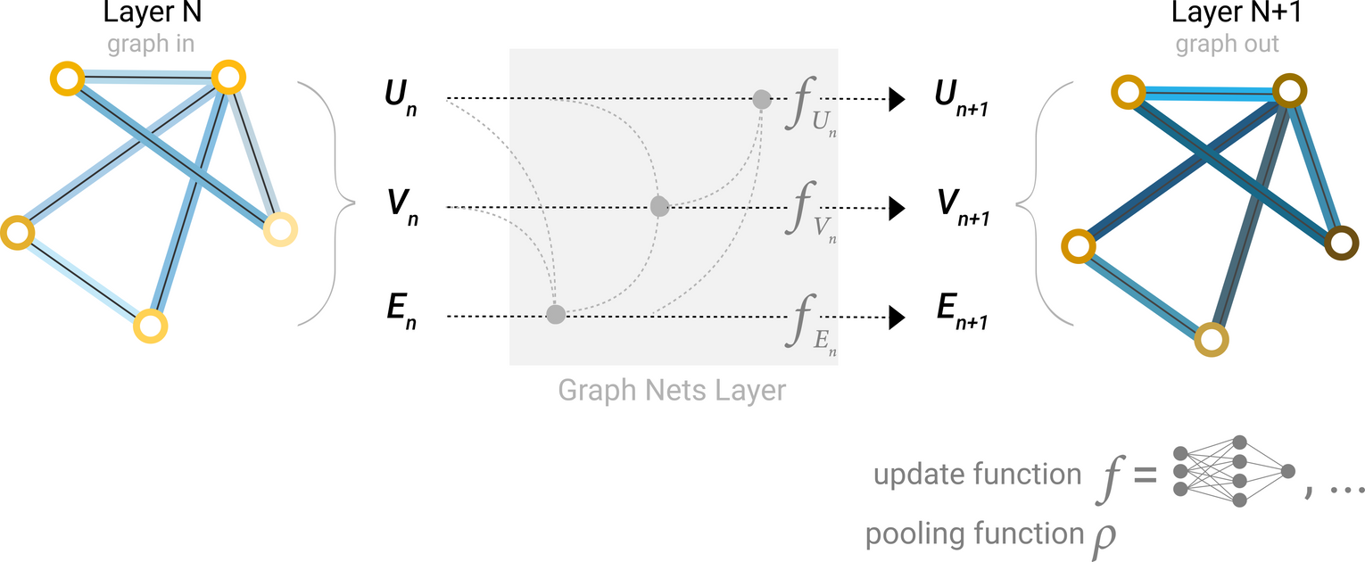
GNN ← Graph Nets architecture schematics + message passing neural network
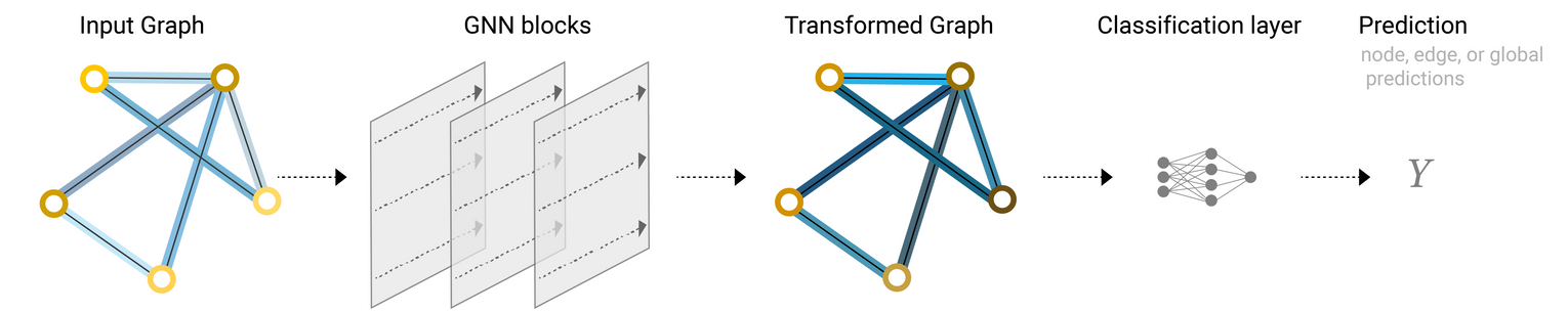
“graph-in, graph-out” : 노드/엣지/global-context의 정보를 입력으로 그래프의 연결성을 변화시키지 않으면서 임베딩을 점진적으로 변환
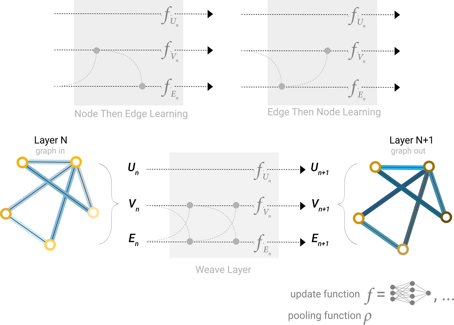
The Simplest GNN
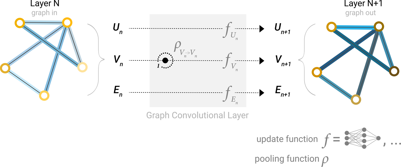
GNN Layer : Graph의 각 component(V = Node, E = Edge, U = Global-context)에 대해 별도의 MLP를 사용
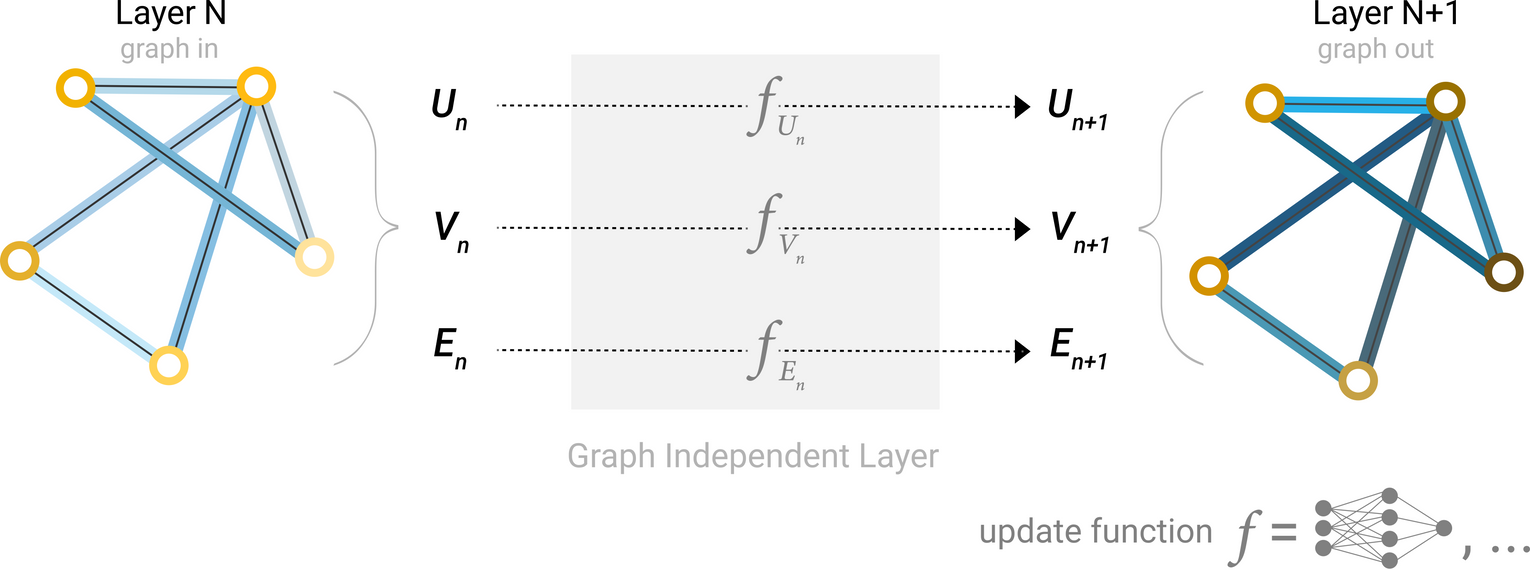
A single layer of a simple GNN. A graph is the input, and each component (V,E,U) gets updated by a MLP to produce a new graph. Each function subscript indicates a separate function for a different graph attribute at the n-th layer of a GNN model.
그래프를 input으로, 동일한 그래프 구조(연결)에 업데이트된 임베딩을 가진 그래프가 output으로 나오게 됨!
GNN Predictions by Pooling Information
각 노드의 업데이트된 임베딩에 대해 선형분류기를 적용하여 node prediction task를 수행할 수 있음
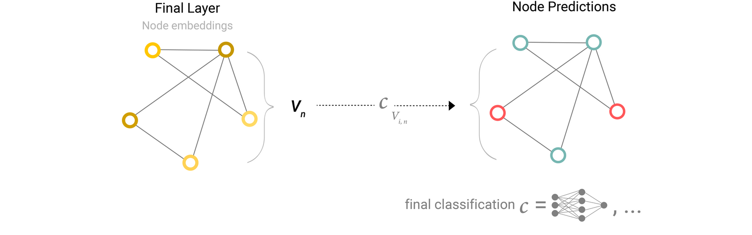
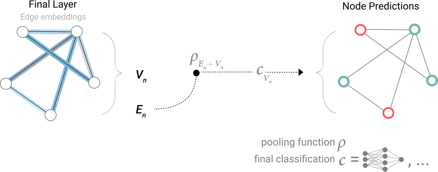
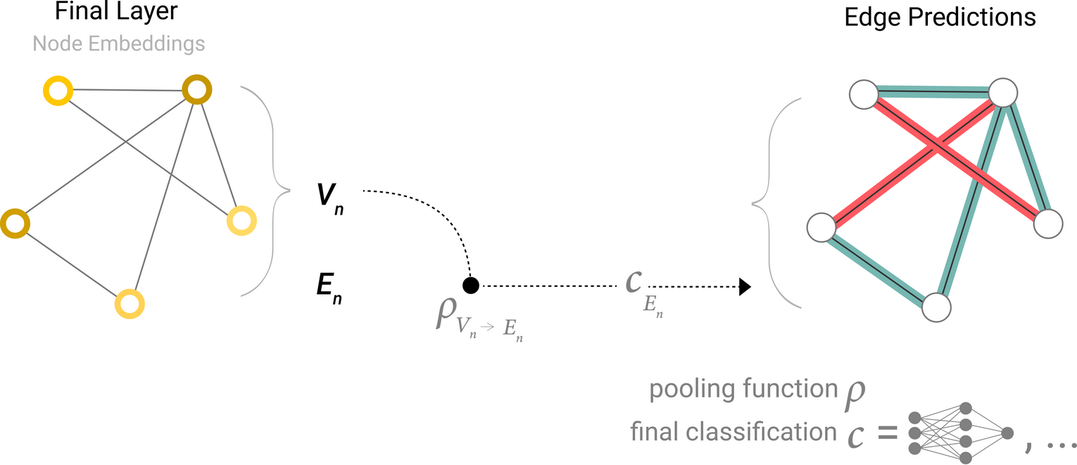
cf. 노드에 대한 정보가 없고, 엣지에 대한 정보는 있는 상황에서 노드에 대한 예측 task를 수행해야할 경우 → 엣지에서 정보를 수집하여 예측을 위해 노드에게 해당 정보를 제공해야함 ⇒ Pooling
2 Steps of Pooling
-
For each item to be pooled, gather each of their embeddings and concatenate them into a matrix. : 풀링할 요소들의 임베딩을 행렬로 concat하여 gathering
-
The gathered embeddings are then aggregated, usually via a sum operation. : 모인 임베딩들을 aggregate(ex. sum)
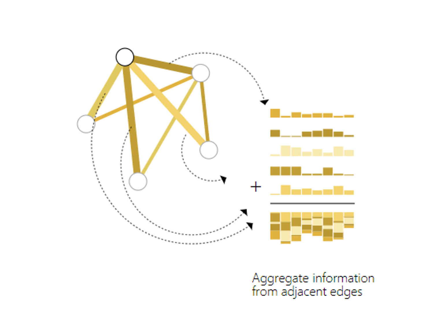
: Pooling operation ⇒ gathering information form edges to node :
Model for predicting binary node information using edge-level features
Model for predicting binary edge-level information using node-level features
Model for predicting binary global property using node-level features
- CNN의 Global average pooling layer와 유사
- 분자특성 예측 task : atomic information + connectivity → toxicity of a molecule

- Classification model 는 다른 differentiable model로 대체 가능
An end-to-end prediction task with a GNN model
An end-to-end prediction task with a GNN model.
- Simplest GNN에서는 각 GNN layer내 그래프 연결성 정보를 활용하지 않음
- 각 노드/엣지는 독립적으로 처리됨
- 예측을 위해 정보를 pooling할 때만 connectivity를 활용
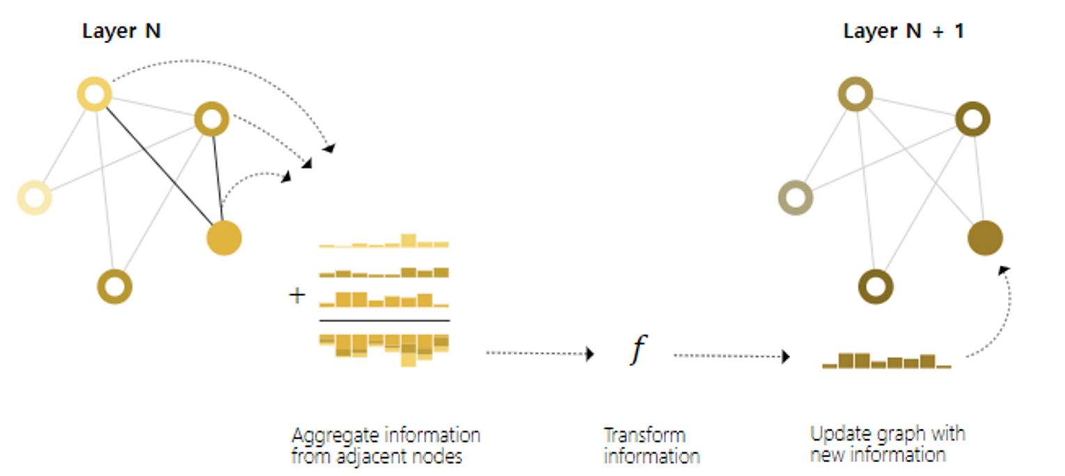
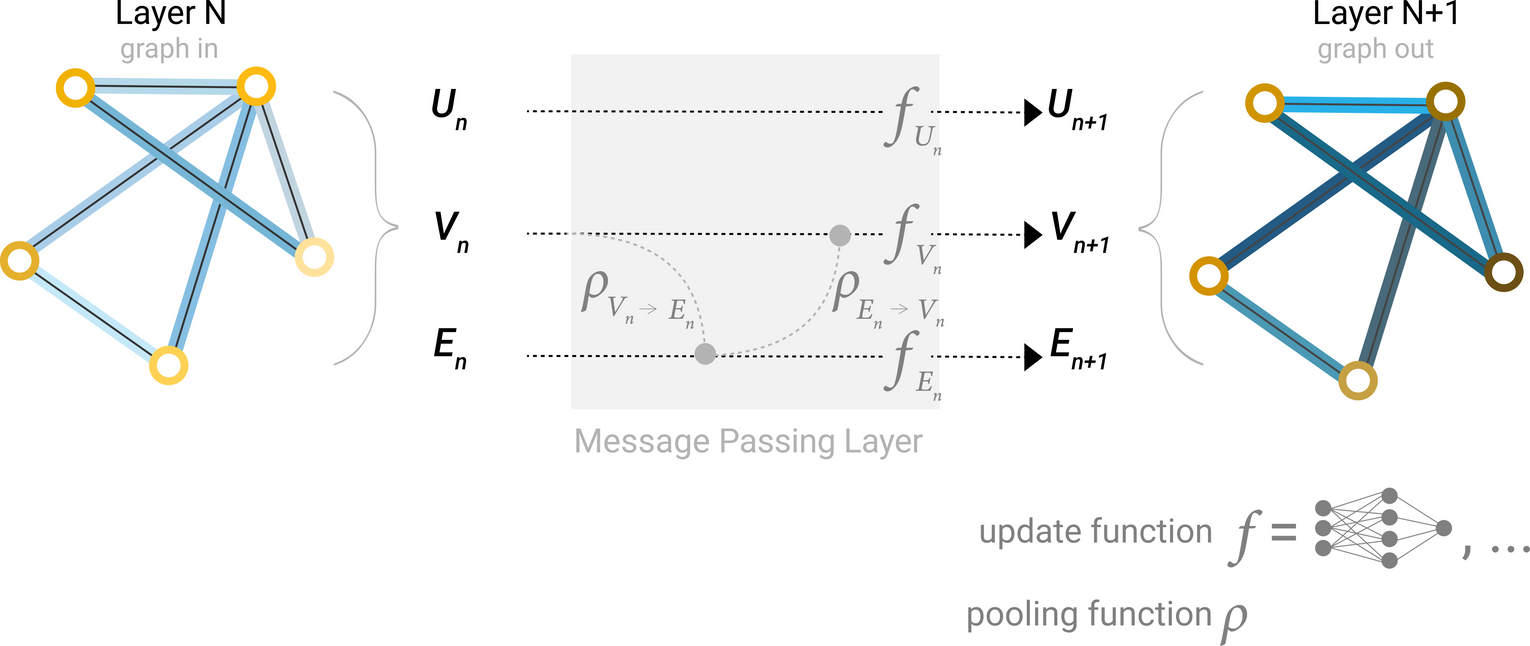
Passing messages between parts of the graph
GNN layer안에서 Pooling을 활용해 graph connectivity를 고려한 임베딩을 만들어 낼 수 있음 ⇒ Message Passing : 이웃하는 노드와 엣지들 사이 정보를 주고받으며 각각의 업데이트에 영향을 줌
Message Passing
- For each node in the graph, gather all the neighboring node embeddings (or messages), which is the function described above. : 함수로 그래프의 각 노드에 대해 모든 인접노드의 임베딩을 모음
- Aggregate all messages via an aggregate function (like sum). : 집계함수로 모인 모든 메세지들을 집계
- All pooled messages are passed through an update function, usually a learned neural network. : 풀링된 모든 메세지는 학습된 NN인 update function으로 전달됨
노드 또는 엣지에 풀링을 각각 적용하는 것과 같이 노드/엣지간의 message passing이 발생할 수 있음
- 그래프의 connectivity 활용
- GNN의 표현력 증가
- Convolution과 비슷한 느낌
- Message passing과 convolution 모두 특정 요소의 값을 업데이트하기위해 이웃의 정보를 집계하여 처리하는 작업
- 차이점 : 이미지에서는 인접 요소의 수가 고정적이지만 그래프는 가변적
- Message passing GNN layer들을 쌓으면, 한 노드는 최종적으로 전체 그래프에 대한 정보를 통합할 수 있음
- layer가 하나 쌓일때마다 정보를 모으는 노드수가 1,2,3,,,hop으로 증가
Schematic for a GCN architecture, which updates node representations of a graph by pooling neighboring nodes at a distance of one degree.
Learning edge representations
*앞선 예시
node에 대한 예측을 수행해야 하는데 edge에 대한 정보만 가지고 있는경우
→ edge정보를 node에 대한 정보로 routing하기 위해 pooling을 해주는 방법 활용
👎) model의 마지막 prediction 단계에 대해서만 적용 가능
⇒ sol💡) message passing을 사용하여 GNN layer내에서 node와 edge사이 정보공유 활성화
👎) edge information과 node information이 같은 차원을 가지고 있다고 보장할 수 없음
⇒ sol💡) 서로의 information space로 mapping하는 linear function을 학습 or concatencate
Architecture schematic for Message Passing layer. The first step “prepares” a message composed of information from an edge and it’s connected nodes and then “passes” the message to the node.
GNN의 설계 요소 중 하나는 node embedding과 edge embedding 중 어떤 것을 먼저 업데이트할지에 대한 결정이 있음
ex. four updated representations that get combined into new node and edge representations: node to node (linear), edge to edge (linear), node to edge (edge layer), edge to node (node layer)
Molecular Graph Convolutions: Moving Beyond Fingerprints
Some of the different ways we might combine edge and node representation in a GNN layer.
Adding global representations
지금까지 설명한 네트워크들의 단점
- message passing을 여러번 적용하더라도 아주 멀리있는 노드들은 서로의 정보를 효율적으로 교환하기 어려움
- i.e. k개의 GNN layer를 쌓으면, k-hop 내의 노드들까지만 정보의 전파가 이루어짐
- node prediction이 멀리 떨어져있는 노드들의 정보에 영향을 받는 경우 문제가 됨
⇒ sol💡) Using global representation of graph(U), i.e. master node or context vector
- Global context vector
- 네트워크 모든 노드, 엣지들과 연결
- information pass의 중간다리 역할
- 그래프 전체의 representaion을 만드는 역할
- 더 풍부하고 복잡한 그래프 representation
Schematic of a Graph Nets architecture leveraging global representations.
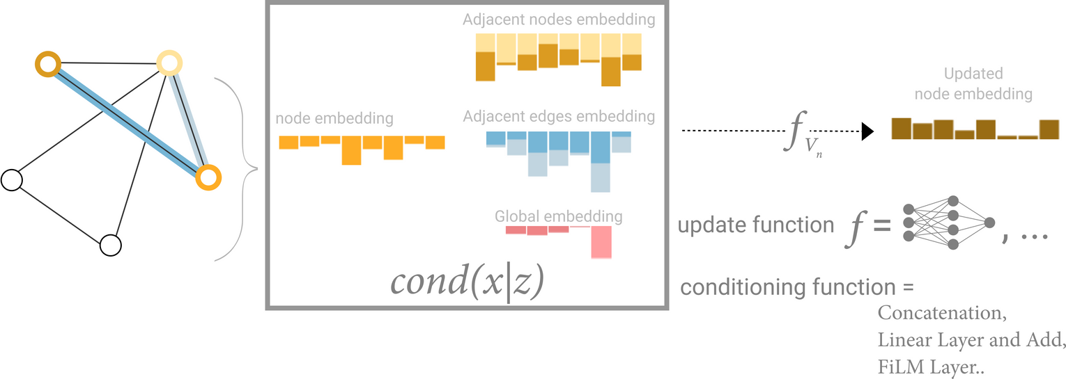
Schematic for conditioning the information of one node based on three other embeddings (adjacent nodes, adjacent edges, global). This step corresponds to the node operations in the Graph Nets Layer.
새로운 노드 임베딩을 만들어낼 때 neighboring nodes, connected edges, global information을 모두 활용할 수도 있지만, conditioning을 통해 일부만 활용할 수도 있음
- concatenate
- learning linear mapping function
- feature-wise modulation layer(featurize-wise attention mechanism)
GNN playground
- Graph-level prediction task
- Leffingwell Odor Dataset
Some empirical GNN design lessons
- a higher number of parameters does correlate with higher performance
- GNNs are a very parameter-efficient model type: for even a small number of parameters (3k) we can already find models with high performance
- models with higher dimensionality tend to have better mean and lower bound performance
- higher dimensionality = higher number of parameter 이기때문에, 위와 동일
- GNN with a higher number of layers will broadcast information at a higher distance
- 노드 하나가 넓은 영역의 그래프의 노드들로부터 정보를 얻어 개별정보가 희석될 위험이 있음 → layer를 쌓을 수록 성능의 boundary가 큼
- the more graph attributes are communicating, the better the performance of the average model
Approach
- neighborhood-based pooling operation
- 그래프 구조에 의존적인 node representation learning
- stochastic graph traversals
- graph information을 얻는 새로운 mechanism들
- Representation Learning on Graphs with Jumping Knowledge Networks
- jumping knowledge (JK) networks는 각 노드의 neighborhood set을 다르게 정의하여 structure-aware representation
- Graph Traversal with Tensor Functionals: A Meta-Algorithm for Scalable Learning
- Graph Traversal via Tensor Functionals(GTTF) : 다양한 graph altorithm을 통해 큰 그래프에서의 효율적인 학습
- Graph Neural Tangent Kernel: Fusing Graph Neural Networks with Graph Kernels
- infinitely wide multi-layer GNNs trained by gradient descent
- Neural Execution of Graph Algorithms
- Representation Learning on Graphs with Jumping Knowledge Networks
Into the Weeds
Other types of graphs (multigraphs, hypergraphs, hypernodes, hierarchical graphs)
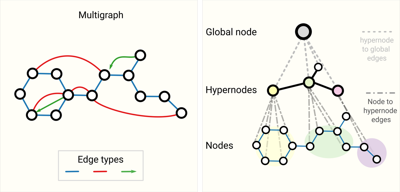
Schematic of more complex graphs. On the left we have an example of a multigraph with three edge types, including a directed edge. On the right we have a three-level hierarchical graph, the intermediate level nodes are hypernodes.
- multigraphs(multi-edge graphs)
- 노드쌍이 여러 type의 edge를 공유
- For example with a social network, we can specify edge types based on the type of relationships (acquaintance, friend, family).
- GNN can be adapted by having different types of message passing steps for each edge type.
- hypernode graphs(nested graphs)
- node represents a graph
- For example, we can consider a network of molecules, where a node represents a molecule and an edge is shared between two molecules if we have a way (reaction) of transforming one to the other
- GNN that learns representations at the molecule level and another at the reaction network level, and alternate between them during training.
- hypergraph
- edge가 2개이상의 노드를 연결
- build a hypergraph by identifying communities of nodes and assigning a hyper-edge that is connected to all nodes in a community.
Sampling Graphs and Batching in GNNs
👎그래프의 경우 노드와 엣지의 수가 고정적이지 않으므로 constant한 batchsize를 만들기 어려움
⇒ 💡 큰 그래프의 필수적인 속성을 보존하는 subgraph를 만들어 batching
-
graph sampling operation
-
그래프에서 노드와 엣지를 sub-selecting하는 과정을 포함하고 context에 매우 의존적
-
Cluster-GCN, GraphSaint 같은 새로운 architecture, training strategy를 만들어내기도 함
⇒ Research Question : How to sample a graph?
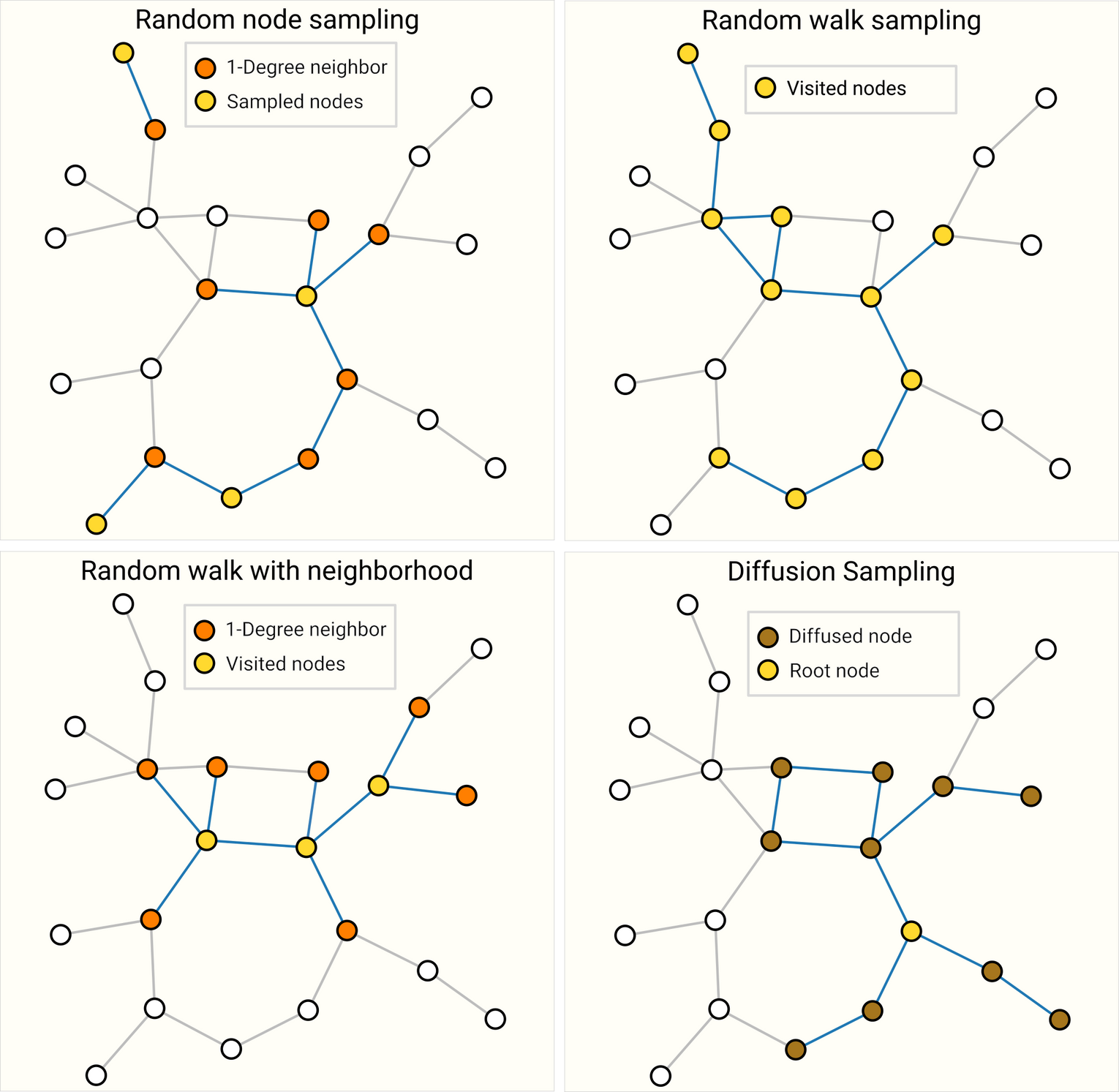
Four different ways of sampling the same graph. Choice of sampling strategy depends highly on context since they will generate different distributions of graph statistics (# nodes, #edges, etc.). For highly connected graphs, edges can be also subsampled.
-
preserving structure at a neighborhood level
- 동일한 숫자의 노드를 random sampling하여 node set을 만들고, edge를 포함해 node set에서 k-hop 이웃 노드들을 추가 ⇒ 이를 개별 그래프처럼 batch 학습에 활용
- The loss can be masked to only consider the node-set since all neighboring nodes would have incomplete neighborhoods.
-
한 노드를 랜덤하게 샘플링한 후 그 노드의 k-hop까지 그래프를 확장한 뒤, 확장된 셋내의 다른 노드를 선택함, 원하는 수의 셋을 만들때 까지 반복
-
Random walk
-
Metropolis algorithm
-
Inductive biases
Relational inductive biases, deep learning, and graph networks
How each graph component (edge, node, global) is related to each other so we seek models that have a relational inductive bias?
- A model should preserve explicit relationships between entities (adjacency matrix) and preserve graph symmetries (permutation invariance).
- node나 edge에의 operation 순서는 상관이 없어야하고, operation이 다양한 input에 작동해야함
Comparing aggregation operations
Aggregation function
- node ordering에 invariant해야함
- differentiable해야함
- 비슷한 input에 대해 비슷한 aggregated output을 만들어내야함
- mean
- when nodes have a highly-variable number of neighbors or you need a normalized view of the features of a local neighborhood
- max
- when you want to highlight single salient(prominent) features in local neighborhoods
- sum
- provides a balance between these two, by providing a snapshot of the local distribution of features, but because it is not normalized, can also highlight outliers
Designing new aggregation operations
- Principal Neighborhood aggregation
- take into account several aggregation operations by concatenating them and adding a scaling function that depends on the degree of connectivity of the entity to aggregate
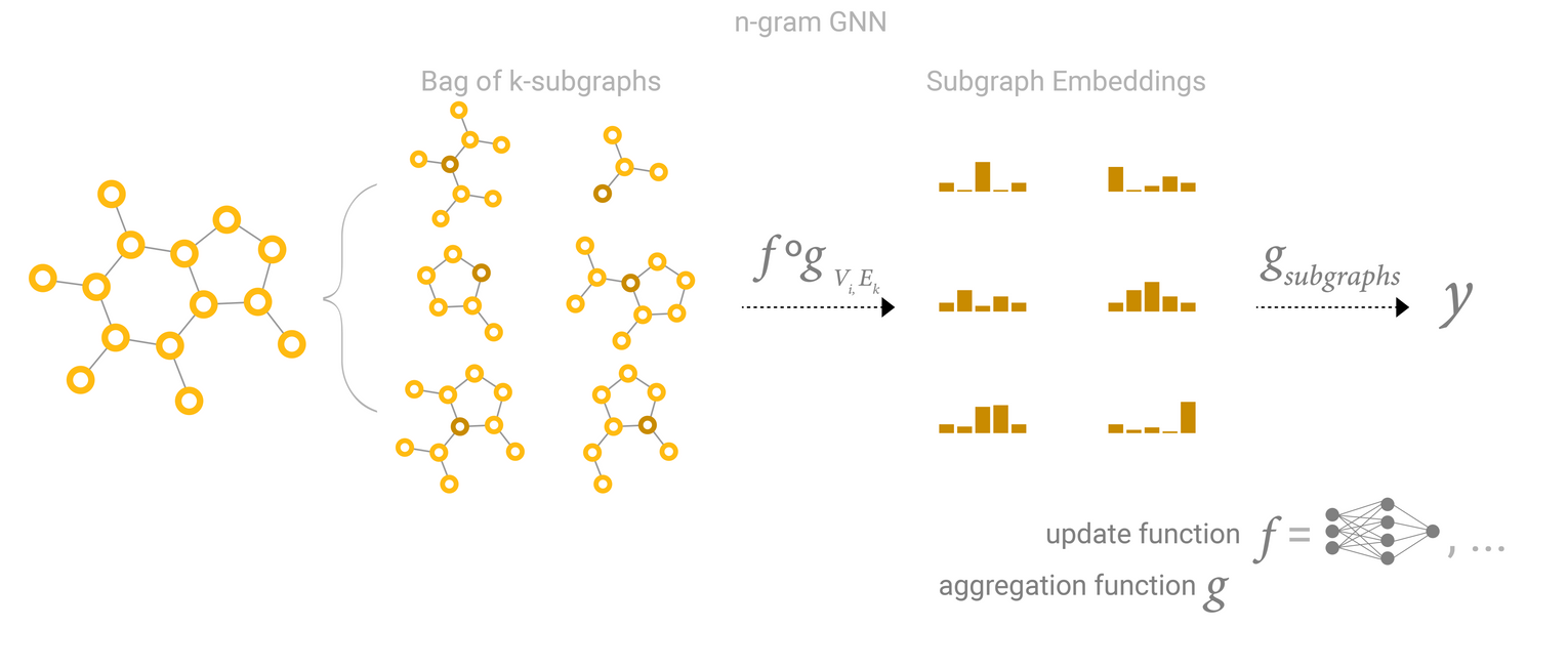
GCN as subgraph function approximators
k layer GNN : 노드로 부터 k-hop의 subgraph에 대한 representation을 학습하는 것
⇒ GCN is collecting all possible subgraphs of size k and learning vector representations from the vantage point of one node or edge
N-Gram Graph: Simple Unsupervised Representation for Graphs, with Applications to Molecules
Edges and the Graph Dual
Edge prediction과 Node prediction task
: an edge prediction task on a graph can be phrased as a node-level prediction on ’s dual.
G의 dual을 얻기 위해, node→edge, edge→node로의 convert가 필요
- Dual Graph?
- Dual-Primal Graph Convolutional Networks
- to solve an edge classification problem on , we can think about doing graph convolutions on ’s dual (which is the same as learning edge representations on )
Graph convolutions as matrix multiplications, and matrix multiplications as walks on a graph
Message passing
- “gathering” all node features values of dimension j that share an edge with
- not updating the representation of the node feature, just pooling neighboring node feature
-
: adjacency matrix,
-
: node feature matrix,
-
: node i와 node k사이 edge의 존재 여부
-
Adjacency matrix 의 sparsity
- matrix multiply-free approach : 가 0인 경우 값을 더할 필요 없음 → 양수 값 retrieval로 해결
- aggregation function으로 sum을 사용할 필요가 없어짐
- matrix multiply-free approach : 가 0인 경우 값을 더할 필요 없음 → 양수 값 retrieval로 해결
위 과정을 여러번 반복하게되면 더 넓은 영역의 정보를 전파할 수 있음
⇒ matrix multiplication is a form of traversing over a graph
: node i와 j사이 길이가 K인 경로의 수**
Graph Attention Networks
Node feature aggregation을 할때 이웃 노드의 중요도 weight를 만들 수 있을까?
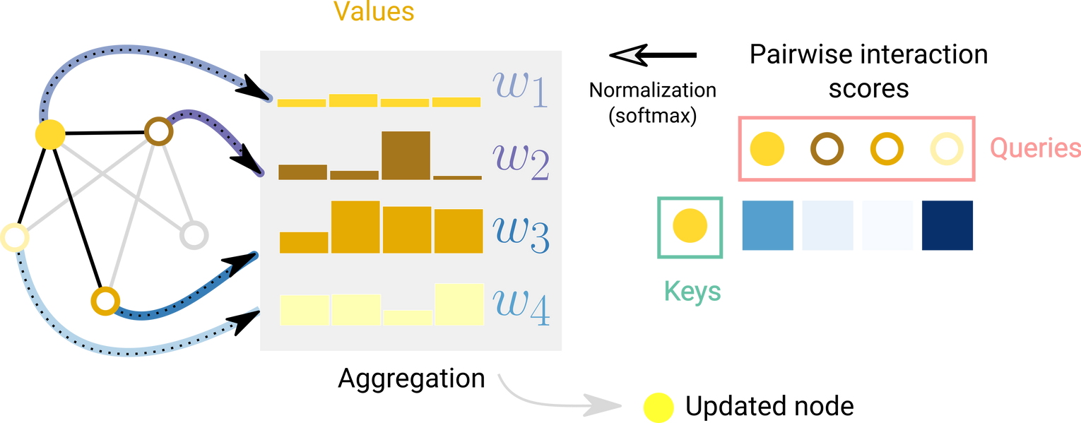
Schematic of attention over one node with respect to it’s adjacent nodes. For each edge an interaction score is computed, normalized and used to weight node embeddings.
Transformers are Graph Neural Networks
- transformers can be viewed as GNNs with an attention mechanism
- transformer models several elements (i.g. character tokens) as nodes in a fully connected graph and the attention mechanism is assigning edge embeddings to each node-pair which are used to compute attention weights →all possible combinations to make a_input :
- The difference lies in the assumed pattern of connectivity between entities, a GNN is assuming a sparse pattern and the Transformer is modelling all connections.
- GNN : adjacency matrix에 대한 연산, aggregation function으로 attention을 사용하느냐, 하지 않느냐의 차이
- Transformer : 모든 노드들의 서로에 대한 가중치 계산 → modelling all connections
Graph explanations and attributions
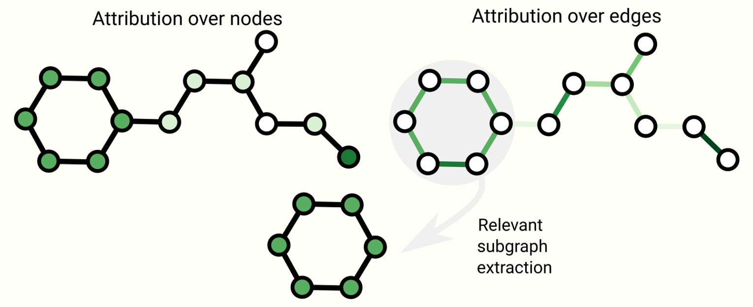
Schematic of some explanability techniques on graphs. Attributions assign ranked values to graph attributes. Rankings can be used as a basis to extract connected subgraphs that might be relevant to a task.
- Graph concept에 따라 달라지는 그래프 explanation에 대한 해결책
- extracting the most relevant subgraph that is important for a task
- Attribution techniques : task에 relevant한 그래프의 part에 대해 importance value를 ranking
- Because realistic and challenging graph problems can be generated synthetically, GNNs can serve as a rigorous and repeatable testbed for evaluating attribution techniques : https://papers.nips.cc/paper/2020/hash/417fbbf2e9d5a28a855a11894b2e795a-Abstract.html
Generative modelling
Graph generation
- Method
- sampling from a learned distribution
- completing a graph given a starting point
- Key Point
- modelling the topology of a graph, which can vary dramatically in size and has terms
- Solution
- Variational Graph Auto-Encoders
- modelling the adjacency matrix directly like an image with an autoencoder framework
- binary classification task : prediction of the presence or absence of an edge
- learns to model positive patterns of connectivity and some patterns of non-connectivity in the adjacency matrix
- build a graph sequentially, by starting with a graph and applying discrete actions such as addition or subtraction of nodes and edges iteratively
- Auto-regressive mode : GraphRNN: Generating Realistic Graphs with Deep Auto-regressive Models
- Optimization of Molecules via Deep Reinforcement Learning
- graph to sequence with grammar elements
- Variational Graph Auto-Encoders