Understanding Convolutions on Graphs

<References>
Understanding Convolutions on Graphs

The Challenges of Computation on Graphs

1. Lack of Consistent Structure

• ex. molecule; 각각 다른 수/종류의 atom을 포함하고 다른 수/종류의 connection을 가짐

2. Node-Order Equivariance

• 원래는 노드에 순서가 없지만, 임의로 부여 ⇒ node-order equivariant

3. Scalability

• very large graph, but sparse

Problem Setting and Notation

• Node Classification: Classifying individual nodes.
• Graph Classification: Classifying entire graphs.
• Node Clustering: Grouping together similar nodes based on connectivity.
• Link Prediction: Predicting missing links.
• Influence Maximization: Identifying influential nodes.

→ 문제 해결에 선행하여 node representation learning이 필요

• Undirected Graph
• $x_v$ : node features for node $v \in V$
• $h_v^{(k)}$ : kth layer(iteration)을 거친 뒤 node v의 representation
• $M_v$ : matrix M에서 node v의 property

Extending Convolutions to Graphs

ordinary convolutions : not node-order invariant

• 이미지의 경우 pixel의 위치에 영향을 받음

⇒ How to generalize convolutions to general graph?

Polynomial Filters on Graphs

• CNN에서 주변 pixel에대해 localized filter를 적용하는 것처럼 주변 노드들에 대해 polynomial filter적용하기

The Graph Laplacian

• A : Adjacency Matrix
• D : Degree Matrix

• L = Graph Laplacian, $n\times n$ matrix

Polynomials of the Laplacian

1. Graph Laplacian을 이해하기 위한 polynomial 만들기
   • polynomial : CNN에서의 필터에 해당하는 느낌
   • coefficient w : 필터의 가중치

이 polynomial의 계수들을 다음의 벡터로 나타낼 수 있다. → $w = [w_0, \dots, w_d]$

• 모든 $w$, $p_w(L)$은 $n \times n$ matrix

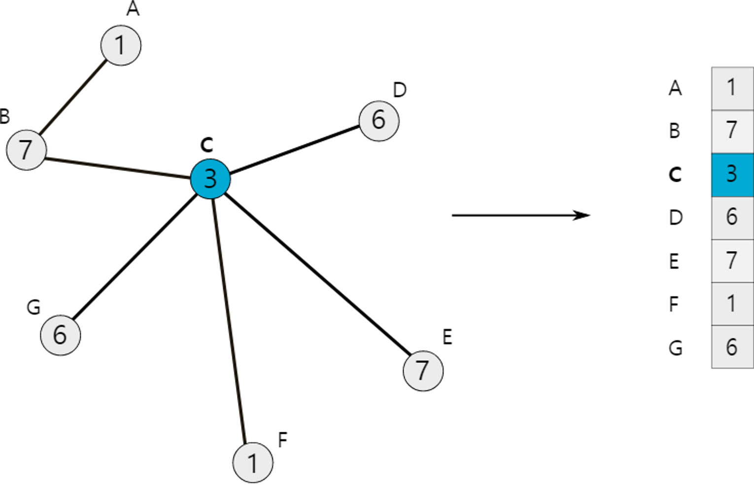
Fixing a node order (indicated by the alphabets) and collecting all node features into a single vector x

• node feature $x_v$가 실수라고 할때, 이를 stacking하여 single vector $x$를 만들 수 있고, 이때 $x \in \mathbb{R}^n$이다.
• feature vector $x$에 대해 polynomial filter $p_w$로 convolution을 적용하면 다음과 같이 나타낼 수 있다.
  $x' = p_w(L)\ x$

💡 1. $p_w(L)= \sum_{i=0}^d w_iL^i$ 에서 계수 $w$가 convolution에 어떤 영향을 미치는가?

• ex1. $w_0 = 1$, $w_i = 0$ for $i$ ≥1 일때

• ex2. $w_1 = 1$, $w_i = 0$ for $i ≠1$ 일때

• Adjacency matrix * x → 이웃 노드들의 feature합계

💡 2. Polynomial의 차수 d는 convolution에 어떤 영향을 미치는가?

• Lemma 5.2 from Wavelets on graphs via spectral graph theory

  Wavelets on graphs via spectral graph theory

  Let $G$ be a weighted graph, $\mathcal{L}$ the graph Laplacian (normalized or non-normalized) and s > 0 an integer. For any two
  vertices m and n, if $d_G(m,n) > s$ then $(\mathcal{L}^s)_{m,n} = 0$.

  Proof.

  

  

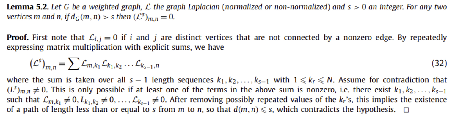
  • s-1 길이의 sequence $k_1, k_2, \dots, k_{s-1}$ with $1≤k_r≤N$
  • 노드 m,n사이의 Laplacian의 s제곱($(\mathcal{L}^s)_{m,n}$)은 m에서 n까지 도달하는 s-1길이의 path들의 노드들사이 Laplacian의 곱의 합(path들간의 합)이라고 할 수 있음
  • 증명하려는 것과 반대로, $(\mathcal{L}^s)_{m,n}$가 non-zero이려면, sum이 진행되는 term(Laplacian matrix의 곱)들 중 적어도 하나가 non-zero이어야 한다.
  • 즉, $\mathcal{L}_{m,k_1} \neq 0, \mathcal{L}_{k_1,k_2} \neq 0, \dots,\mathcal{L}_{k_{s-1},n} \neq 0.$ 인 $k_1, k_2, \dots, k_{s-1}$(path)이 존재한다. ⇒ 노드 m,n사이에 길이가 s인 path가 존재한다.
  • 반복되는 노드를 제거할경우, “노드 m,n사이에 길이가 s보다 작은 path가 존재한다”고 정리할 수 있다.
  • 즉, $(\mathcal{L}^s)_{m,n} = 0$ 이려면, 노드 m,n사이에 길이가 s보다 짧은 path가 존재하지 않는다. ⇒ 두 노드 사이 거리는 s보다 크다.

다시 돌아와서 Polynomial의 차수 d가 convolution에 미치는 영향에 대해 보면,

$x'$를 얻기 위해 $x$를 차수가 $d$인 polymonial $p_x(L)$로 대체하면,

• 노드 v에서의 convolution은 d hop보다 멀지 않은 노드들에 대해서만 적용됨
  • localized polynomial filters, d의 크기에 따라 localization의 정도 변동

ChebNet

위에서 사용했던 polynomial filter는 다음과 같이 정의됨

ChebNet에서는 polynomial filter를 다음의 형태로 수정하여 사용

• $T_i$ : i차의 1종 체비세프 다항식
  • 체비세프 다항식
• $\tilde{L}$ : L의 가장 큰 eigen value를 사용해 정의된 normalized Laplacian
  $\tilde{L} = \frac{2L}{\lambda_{\text{max}}(L)}-I_n$
  • L → positive semi-definite : L의 모든 eigenvalue들은 0보다 작지 않다.
  • $\lambda_{\text{max}} > 1$ 이라면, L의 제곱들은 급격하게 크기가 커지게 되는데, L을 효율적으로 scale-down한 $\tilde{L}$의 경우 eigenvalue들이 [-1,1]의 구간에 있음을 보장하여 제곱값의 크기가 끝없이 커지는 것을 막는다.
    • unnormalized Laplacian $L$에 대해 높은 차원의 계수의 크기 제한
    • normalized Laplacian $\tilde{L}$에 대해서는 더 큰 값의 계수 허용
  • chebyshev polynomial → interpolation을 수치적으로 안정적이게 만드는 특성

Polynomial Filters are Node-Order Equivariant

Polynomial filter

• node order에 independent ← $p_w$의 차원이 1이고, x가 이웃 노드의 feature를 aggregate한 value인 경우를 떠올리면 이해하기 쉬움(ex. 합계는 순서와 상관이 없음)
• proof. permutation matrix $P$ : 정사각 이진 행렬, 각 행에 값이 1인 요소가 하나 있고, 나머지는 0의 값을 가짐. 다른 matrix $A$ 를 곱해주었을 때 $A$의 각 row를 permutating해주는 것과 같은 효과라고 이해하면 됨.(=행 교환을 수행하는 행렬)
  $PP^T =P^TP = I_n$
  function $f$ : node-order equivariant
  $f(Px) = Pf(x)$
  permutation matrix $P$를 활용해 새로운 node-order를 만들어내면, 다음과 같은 변환이 수행된다.
  $\begin{aligned} x &\rightarrow Px\\L&\rightarrow PLP^T \\ L^i &\rightarrow PL^iP^T \end{aligned}$
  $f(x) = p_w(L)x$ 와 같은 polynomial filter가 있을 때, 다음과 같이 정리할 수 있다.
  $\begin{aligned} f(Px) &= \sum^{d}_{i=0}w_i(PL^iP^T)(Px)\\ &=P\sum^{d}_{i=0}w_iL^ix\\&=Pf(x) \end{aligned}$

Embedding Computation

• $K$ different polynomial filter layer
  • $k^{th}$ layer의 learnable weights $w^{(k)}$

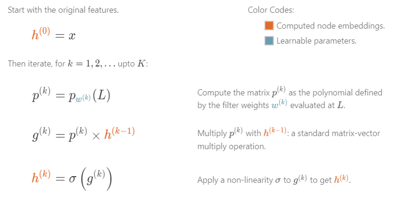
• $w^{(k)}$의 weight를 가진 polynomial filter를 $L$에 적용하여 matrix $p^{(k)}$를 계산
• $p^{(k)}$에 $h^{(k-1)}$를 곱해 $g^{(k)}$를 계산
• $g^{(k)}$에 non-linearity $\sigma$를 적용하여 $h^{(k)}$를 계산
• CNN에서의 weight-sharing(동일한 필터를 여러 grid에 적용)과 마찬가지로, 다른 노드들에 같은 weight를 가진 filter를 적용

Modern Graph Neural Networks

• $w_1 = 1$, 나머지 $w_i$들은 모두 0
• $p_w(L) = L$
• $p_w$의 차원 d ⇒ 얼마나 localized된 필터를 사용할 것인가

• Aggregation : 바로 이웃하는 노드 feature $x_u$들을 aggregate
• Combination : 자기자신의 feature $x_v$를 합침

💡 Polynomial filter를 사용해 가능한 것과 별개로 다른 종류의 “Aggregation”, “Combination” 를 사용하면 어떨까?

• Aggregation이 node-order equivariant하다면, convolution 전체가 node-order equivariant하다.
• 바로 이웃하는 노드들 사이의 “message-passing”과정이라고 이해할 수 있다.
• 1-hop localized convolution을 K번 반복하면, K-hop만큼 멀리에 있는 노드들까지 receptive field를 늘릴 수 있다.

Embedding Computation

Message-passing을 backbone으로 하는 많은 GNN Architecture들

• Graph Convolutional Networks (GCN)
• Graph Attention Networks (GAT)
• Graph Sample and Aggregate (GraphSAGE)
• Graph Isomorphism Network (GIN)

1. Graph Convolutional Networks (GCN)

   

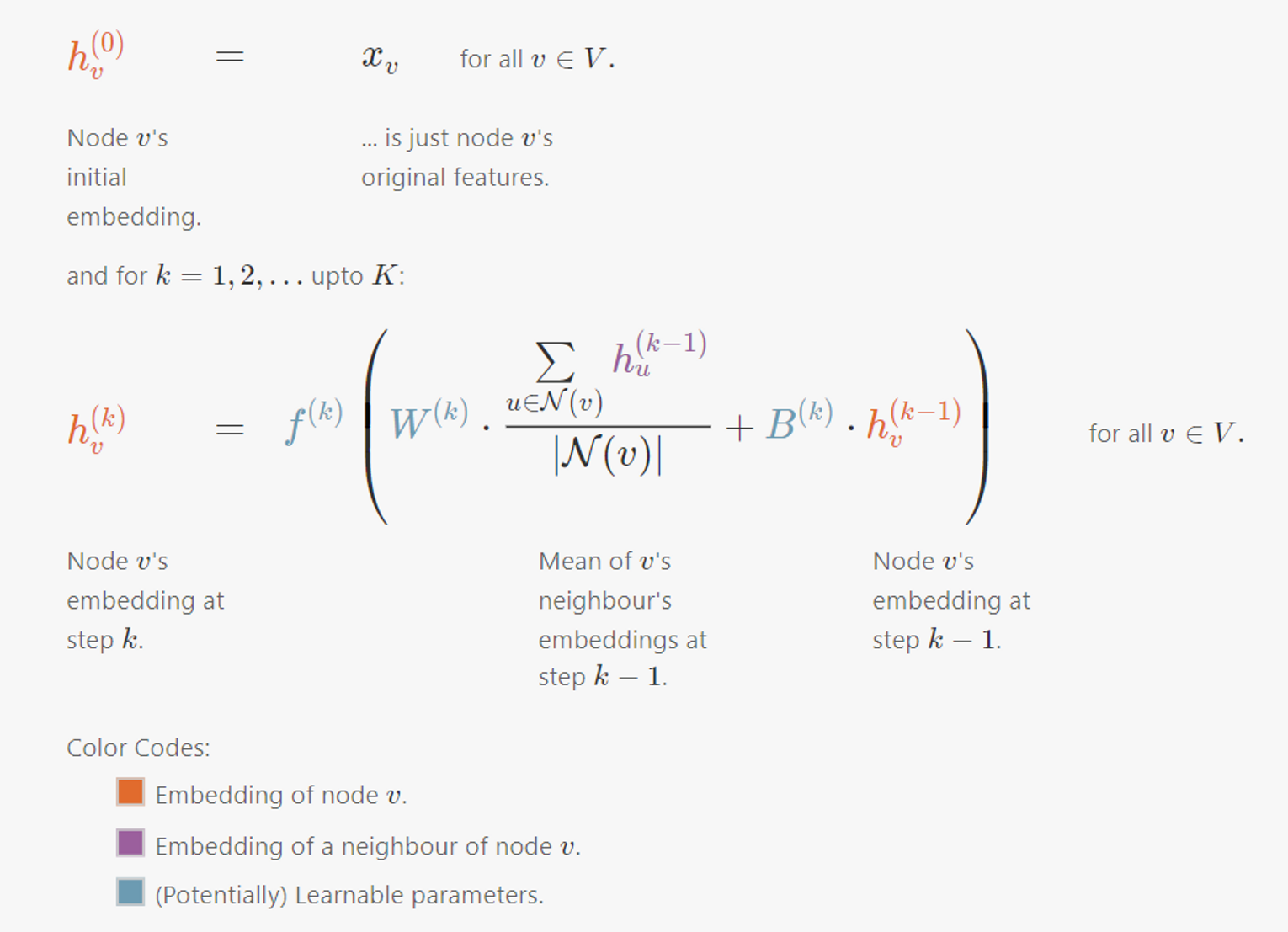
   • 각 k 단계별로 학습가능한 function $f^{(k)}$, matrics $W^{(k)}$, $B^{(k)}$는 모든 노드들에 걸쳐 공유됨

2. Graph Attention Networks (GAT)

   

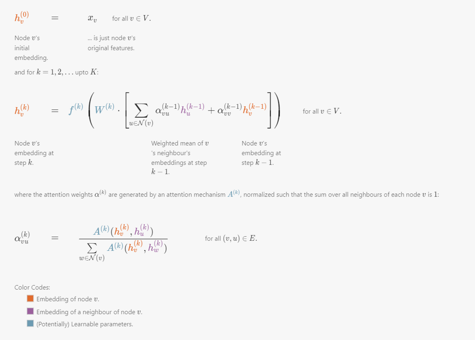
   • 각 k 단계별로 학습가능한 function $f^{(k)}$, matrics $W^{(k)}$, $B^{(k)}$, Attention $A^{(k)}$는 모든 노드들에 걸쳐 공유됨
   • multi-head attention

3. Graph Sample and Aggregate (GraphSAGE)

   

   • 각 k 단계별로 학습가능한 function $f^{(k)}$, matrics $W^{(k)}$, $\text{AGG}$는 모든 노드들에 걸쳐 공유됨

   • $\text{AGG}$의 선택

     • Mean(GCN과 유사)
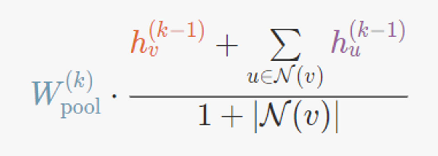
     • Dimension-wise Maximum
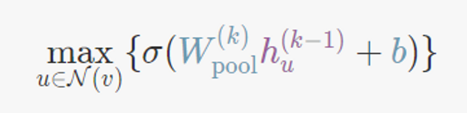
     • LSTM (after ordering the sequence of neighbours)

   • neighbourhood sampling : 노드의 이웃노드 수에 관계 없이 고정된 수의 노드들을 random sampling하여 GraphSAGE가 매우 큰 그래프에도 적용될 수 있게됨, Node embedding의 variance는 증가

4. Graph Isomorphism Network (GIN)

   

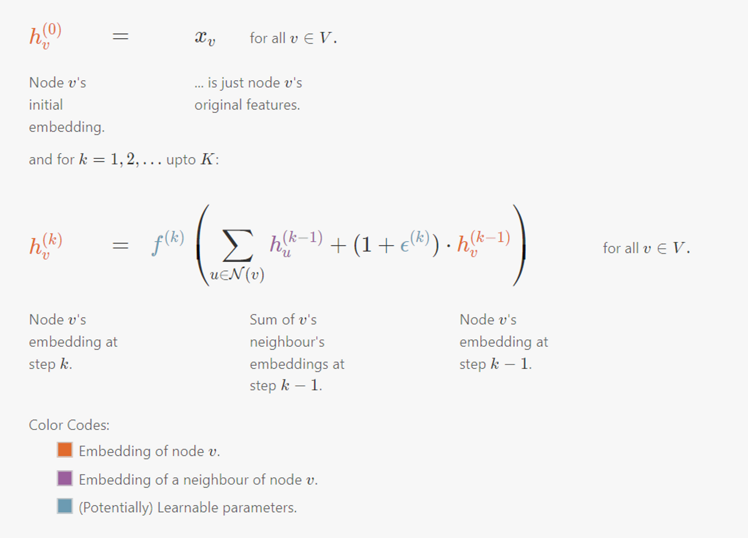
   • 각 k 단계별로 학습가능한 function $f^{(k)}$, real-valued parameter $\epsilon^{(k)}$는 모든 노드들에 걸쳐 공유됨

Prediction

• 최종적으로 계산된 embedding을 사용해 각 노드에 대한 prediction을 만들어내는 방법은 다음과 같다.

• $\text{PREDICT}$ : 또다른 Neural Net, 각 GNN을 학습할 때 같이 학습

From Local to Global Convolutions

message passing을 반복적으로 수행하여 그래프 전체에서 한 노드로 정보가 모일 수 있지만, 직접적으로 global convolution을 수행하는 방법이 있음

Spectral Convolutions

💡 feature vector $x$에 대해, Laplacian $L$을 사용해 $G$에 관해 $x$가 얼마나 smooth한지 quantify할 수 있음

$\sum_{i=1}^{n} x^2_i = 1$을 만족하는, 즉, normalize된 $x$에 대해

Rayleigh quotient를 정의하면 다음과 같다.

• Laplacian matrix의 value가 0이면 두 노드는 인접하지 않음.
• $L = D-A$
• 인접한 노드 feature의 차이의 제곱으로 정리할 수 있음
• = Smoothness
• 인접한 노드 feature가 유사하면 $R_L(x)$ 값이 작아짐

Laplacian matrix $L$

• Real, symmetric matrix
• eigenvalues : $\lambda_1 ≤ \dots ≤ \lambda_n$이
• 이에 대응하는 $u_1, \dots, u_n$는 orthonormal

• L의 eigenvectors → successively less smooth
• L의 eigenvalue들을 “spectrum”이라고 할때, L의 spectral decomposition은
  $L = U\Lambda U^T$
  • $\Lambda$ : 정렬된 eigenvalue들의 대각행렬 = $\begin{bmatrix}\lambda_{1} & & \\ & \ddots & \\ & & \lambda_{n}\end{bmatrix}$
  • $U$ : eigenvector들의 matrix, 정렬된 eigenvalue에 대응 = $\begin{bmatrix}u_1 \dots u_n\end{bmatrix}$

eigenvector들은 orthonormality condition을 만족 : $U^TU = I$

eigenvector들은 $\mathbb{R}^n$의 basis로 다음과 같이 linear combination으로 feature vector $x$를 나타낼 수 있음

• $\hat{x}$ : $\begin{bmatrix}x_0 \dots x_n\end{bmatrix}$의 coefficient, spectral representation of vector $x$
• orthonormality condition을 $x = U\hat{x}$에 적용하면, natural representation $x$와 spectral representation $\hat{x}$ 사이 변환식으로 정리할 수 있음

Embedding Computation

• $k$ layers → each layers’ learnable parameter $\hat{w}^{(k)}$ = filter weights
• spectral representation을 계산하는데 필요한 eigenvector의 수 = $m$ = 각 layer에 필요한 weight의 수
• spectral domain에서 convolution을 적용하면 direct convolution보다 더 적은 파라미터를 사용해도 됨
• Laplacian eigenvector들의 smoothness덕분에, spectral representation을 사용하면 자연스럽게 주변 노드들이 유사한 representation을 갖도록하는 inductive vias를 강화할 수 있음
• node feature가 1d라고 할 때, 각 layer의 output은 node representation $h^{(k)}$의 벡터로, 각 행은 node의 representation을 의미
  $h^{(k)} = \begin{bmatrix}h^{(k)}_{1}\\ \vdots \\ h^{(k)}_{n}\end{bmatrix} \quad \scriptsize \text{for each } k = 0,1,2,\dots \text{up to }K$

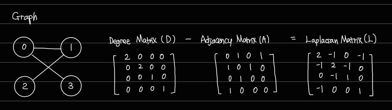
Graph $G$

• adjacency matrix $A$
• degree matrix $D$
• Lapalcian $L = D-A$

• $\Lambda$ : 정렬된 eigenvalue들의 대각행렬 = $\begin{bmatrix}\lambda_{1} & & \\ & \ddots & \\ & & \lambda_{n}\end{bmatrix}$
• $U$ : eigenvector들의 matrix, 정렬된 eigenvalue에 대응 = $\begin{bmatrix}u_1 \dots u_n\end{bmatrix}$

1. Start with original feature $h^{(0)} = x$
2. Iterate, for k=1,2,… upto K

   1. Convert previous feature $\color{#FE6100}{h}^{(k - 1)}$ to its spectral representation $\hat{h}^{(k - 1)}$

      : spectral representation으로 변환하기

      $\hat{h}^{(k - 1)}= U^T_mh^{(k - 1)}$

   2. Convolve with filter weights ${\color{#4D9DB5} \hat{w}^{(k)}}$ in the spectral domain to get ${\hat{g}^{(k)}}$, $\odot$  = element-wise multiplication

      : weight가 $\hat{w}^{(k)}$인 filter로 spectral domain에서의 convolution적용

      $\hat{g}^{(k)} = \hat{w}^{(k)} \odot \hat{h}^{(k-1)}$

   3. Convert $\hat{g}^{(k)}$ back to its natural representation ${g}^{(k)}$

      : spectral → natural

      $g^{(k)} = U_m\hat{g}^{(k)}$

   4. Apply a non-linearity $\sigma$ to ${g}^{(k)}$ to get $\color{#FE6100} {h}^{(k)}$

      $h^{(k)} = \sigma (g^{(k)})$

Spectral Convolutions are Node-Order Equivariant

Laplacian polynomial filter의 node equivariant 증명에서 보인 것과 유사한 접근으로 증명 가능

• proof. node order의 변경 : permutation matrix $P$( = 행 교환을 수행하는 행렬)와의 내적 그에 따라 다음과 같은 식의 변경 발생
  $\begin{aligned} x &\rightarrow Px\\A&\rightarrow PAP^T\\L&\rightarrow PLP^T \\ U_m &\rightarrow PU_m \end{aligned}$
  embedding computation에는 다음과 같은 변경
  $\begin{aligned} \hat{x} &\rightarrow(PU_m)^T(Px) = U^T_mx = \hat{x}\\ \hat{w}&\rightarrow (PU_m)^T(Pw) = U^T_mw = \hat{w}\\ \hat{g}&\rightarrow \hat{g} \\ g &\rightarrow (PU_m)\hat{g} = P(U_m\hat{g}) = Pg \end{aligned}$
  $\sigma$ 가 elemnetwise 방향으로 적용되므로
  $f(Px) = \sigma(Pg) = P \sigma(g) = Pf(x)$
  와 같이 정리할 수 있다.

+) spectral의 $\hat{x}, \hat{w}, \hat{g}$는 node permutation이 되더라도 변하지 않는다.

Spectral convolution의 단점

1. $L$로부터 eigenvector matrix $U_m$을 계산해야 하는데, 아주 큰 그래프에 대해서 이것이 불가능해질 수도 있다.
2. U_m 을 계산해내더라도, global convolution을 계산하는 것이 $U_m$, $U^T_m$ 을 반복적으로 곱해주어야해서 비효율적일 수 있다.
3. 학습된 필터가 input그래프의 Laplacian L의 spectral decomposition에 관한것이기 때문에 그래프 specific해서 다른 구조를 가진 그래프에 transfer하여 적용하기 어렵다.

Global Propagation via Graph Embeddings

graph-level information을 node와 edge의 정보를 pooling함으로써 전체 그래프의 embedding을 계산하고, 그래프 embedding을 사용해 노드 embedding을 업데이트하여 전체 그래프의 embedding을 계산 → Relational inductive biases, deep learning, and graph networks

• spectral convolution이 잡아낼 수 있는 그래프의 topology를 무시하는 경향이 있음

Learning GNN Parameters

embedding computations → completely differentiable ⇒ end-to-end training이 가능

Task에 따른 Loss function $\mathcal{L}$

Node Classification

• $\hat{y}_{vc}$ : node v가 class c로 예측될 확률
• cross-entropy loss
• semi-supervised setting에서는 다음과 같이 정의할 수 있음
  $\mathcal{L}_G = \frac{\sum_{v \in \text{Lab}(G)}\mathcal{L}(y_v,\hat{y}_v)}{|\text{Lab}(G)|}$
  • $\text{Lab}(G)$ : labelled nodes에 대해서만 loss계산

Graph Classification

node representation을 aggregate하여 전체 그래프에 대한 representation생성

• Pooling
  $h_G = \text{PREDICT}_G(\text{AGG}_{v \in G}(\{h_v\}))$
  • SortPool (An End-to-End Deep Learning Architecture for Graph Classification) : 그래프의 정점들을 sort하여 고정된 크기의 node-order invariant한 그래프 representation을 만들고, 일반적인 NN architecture에 적용
  • DiffPool (Hierarchical Graph Representation Learning with Differentiable Pooling) : 정점을 클러스터링하고, 노드 대신 클러스터로 coarser graph를 만들고, coarser graph에 GNN을 적용한다. 하나의 클러스터만 남을때 까지 반복
  • SAGPool (Self-Attention Graph Pooling) : GNN을 적용해 node score를 학습하고, 상위 score를 가진 노드만 남기고 나머지는 버림. 하나의 노드만 남을때까지 반복

Link Prediction

adjacent, non-adjacent한 노드 쌍을 sampling하여 이 벡터 쌍을 연결 유무를 예측하기 위해 사용

• $e_{vu}$ : node v와 u사이에 edge 가 있으면 1, otherwise 0

Others

NLP에서 ELMo나BERT에서 적용된 테크닉을 GNN에 적용해볼 수 있음

• local graph properties (eg. node degrees, clustering coefficient, masked node attributes)
• global graph properties (eg. pairwise distances, masked global attributes)

인접 노드가 비슷한 embedding을 갖도록 하기 위한 self-supervised technique 중 node2vec이나 DeepWalk등 random-walk와 유사한 접근을 하기도 함

• $N_R(v)$ : node v에서 시작하여 random-walk를 통해 방문한 node들의 multi-set

아주 큰 그래프에 대해서는 Noise Contrastive Estimation을 적용하기도 함

• Noise-Contrastive Estimation of Unnormalized Statistical Models, with Applications to Natural Image Statistics
• Learning word embeddings efficiently with noise-contrastive estimation