210707 kaggle 실습
House Prices - Advanced Regression Techniques
- 주어진 관련 데이터를 토대로 집 값을 예측하는 회귀 분석
- 기술 및 분석 능력을 통해 보다 정확한 예측 성능을 기대
- 데이터 전처리를 통해 결측치 처리
-시각화
-모델 앙상블을 통해 예측 성능 향상
참고 블로그: https://jamm-notnull.tistory.com/12
데이터 로드
import pandas as pd
import numpy as np
from scipy.stats import norm
%matplotlib inline
import matplotlib.pyplot as plt
import seaborn as sns
import warnings; warnings.simplefilter('ignore')train=pd.read_csv('./data_in/house/train.csv', index_col='Id')
test=pd.read_csv('./data_in/house/test.csv', index_col='Id')
submission=pd.read_csv('./data_in/house/sample_submission.csv', index_col='Id')
data=train
print(train.shape, test.shape, submission.shape)(1460, 80) (1459, 79) (1459, 1)
데이터 분석
1. 타겟 변수 확인
figure, (ax1, ax2) = plt.subplots(nrows=1, ncols=2)
figure.set_size_inches(14,6)
sns.distplot(data['SalePrice'], fit=norm, ax=ax1)
sns.distplot(np.log(data['SalePrice']+1), fit=norm, ax=ax2)
#데이터에 0이 있을 수 있기 때문에 1을 더해줌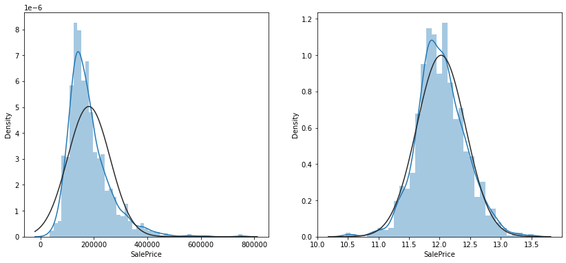
- 분포가 오른쪽으로 길게 있는 것을 알 수 있다
- 오른쪽 꼬리 부분은 데이터가 적어 학습이 잘 안될 가능성이 있음
- 해당 변수에 로그를 취하면 비대칭도가 줄어들고, 정규분포에 가깝게 데이터가 분포하게 된다
2. 변수 간 상관관계 확인
corr=data.corr()
top_corr=data[corr.nlargest(40,'SalePrice')['SalePrice'].index].corr()
figure, ax1 = plt.subplots(nrows=1, ncols=1)
figure.set_size_inches(20,15)
sns.heatmap(top_corr, annot=True, ax=ax1)
- 변수 OverallQual이라는 변수가 상관계수 0.79로 타겟변수와 가장 큰 상관관계
- 전반적으로 이 변수가 증가하면 집값 증가
<상관 관계 분석>
- 변수 A와 B가 있을 때 변수 A의 값이 커질 때 B값도 커지면 둘은 양의 상관관계를 가짐-
- 반대로 A가 커질 때 B가 작아지면 음의 상관관계
- 서로 영향이 없으면 상관관계가 0
- 상관 계수란 이 상관 관계를 측정하는 값으로 주로 피어슨 상관계수를 이용해 분석
- 피어슨 상관계수: 두개의 수치값들의 집합이 있을 때 이 두개의 수치값들은 각각의 순서쌍에 대해서 연결관계가 있다고 할 때 두 수치값이 서로 관련이 있는지를 확인하는 방법
sns.regplot(data['GrLivArea'], data['SalePrice'])- 두 번째로 큰 상관 계수를 가진 GrLivArea의 그래프
- 전체적으로 이 값이 증가하면 집 값도 증가
- 위 그래프에서 오른 쪽 아래의 두 점은 전혀 다른 결과를 보여준다
- 이런 데이터를 이상치로 간주하고 삭제하는 것이 머신러닝의 정확도를 높이는 방법 중 하나
train=train.drop(train[(train['GrLivArea']>4000) & (train['SalePrice']<300000)].index)Ytrain=train['SalePrice'] #타겟 변수
train=train[list(test)]
all_data=pd.concat((train, test), axis=0)
print(all_data.shape)
Ytrain=np.log(Ytrain+1) #위에서 했던 것 처럼 로그 씌움(2917, 79)
3. 전체 데이터에서 결측치 확인
cols=list(all_data)
for col in list(all_data):
    if (all_data[col].isnull().sum())==0:
        cols.remove(col)
    else:
        pass
print(len(cols))
print(cols)#결측치가 있는 변수명들 출력
34
['MSZoning', 'LotFrontage', 'Alley', 'Utilities', 'Exterior1st', 'Exterior2nd', 'MasVnrType', 'MasVnrArea', 'BsmtQual', 'BsmtCond', 'BsmtExposure', 'BsmtFinType1', 'BsmtFinSF1', 'BsmtFinType2', 'BsmtFinSF2', 'BsmtUnfSF', 'TotalBsmtSF', 'Electrical', 'BsmtFullBath', 'BsmtHalfBath', 'KitchenQual', 'Functional', 'FireplaceQu', 'GarageType', 'GarageYrBlt', 'GarageFinish', 'GarageCars', 'GarageArea', 'GarageQual', 'GarageCond', 'PoolQC', 'Fence', 'MiscFeature', 'SaleType']
#집에 해당 시설물이 없는 경우(범주형 변수)'None'으로 채움
for col in ('PoolQC', 'MiscFeature', 'Alley', 'Fence', 'FireplaceQu', 'GarageType', 'GarageFinish', 'GarageQual', 'GarageCond', 'BsmtQual', 'BsmtCond', 'BsmtExposure', 'BsmtFinType1', 'BsmtFinType2', 'MasVnrType', 'MSSubClass'):
    all_data[col] = all_data[col].fillna('None')

#집에 해당 시설물이 없는 경우(수치형 변수) 0으로 채움
for col in ('GarageYrBlt', 'GarageArea', 'GarageCars', 'BsmtFinSF1', 'BsmtFinSF2', 'BsmtUnfSF','TotalBsmtSF', 'BsmtFullBath', 'BsmtHalfBath', 'MasVnrArea','LotFrontage'):
    all_data[col] = all_data[col].fillna(0)

#해당 시설물이 없다고 보기 힘든 경우 해당 열의 최빈 값으로 채움
for col in ('MSZoning', 'Electrical', 'KitchenQual', 'Exterior1st', 'Exterior2nd', 'SaleType', 'Functional', 'Utilities'):
    all_data[col] = all_data[col].fillna(all_data[col].mode()[0])

print(f"Total count of missing values in all_data : {all_data.isnull().sum().sum()}")
Total count of missing values in all_data : 0
- 위에서 출력한 결측치가 있는 변수의 결측 값들을 채워준다
- 범주형 변수의 경우 'None', 수치형 변수의 경우 0, 해당 시설물이 없다고 보기 힘든 경우에는 해당 열의 최빈 값으로 채운다
4. 데이터 분석
- 총 가용면적
figure, ((ax1, ax2), (ax3, ax4)) = plt.subplots(nrows=2, ncols=2)
figure.set_size_inches(14,10)
sns.regplot(data['TotalBsmtSF'], data['SalePrice'], ax=ax1)#모두 합한 총 면적 (오른쪽 아래)
sns.regplot(data['1stFlrSF'], data['SalePrice'], ax=ax2)#1층 면적
sns.regplot(data['2ndFlrSF'], data['SalePrice'], ax=ax3)#2층 면적
sns.regplot(data['TotalBsmtSF'] + data['1stFlrSF'] + data['2ndFlrSF'], data['SalePrice'], ax=ax4)#지하실 면적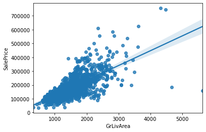
- 오른 쪽 아래가 총 면적
- 결과를 보면 총 면적이 증가하면 집 값이 비싸짐을 알 수 있다
all_data['TotalSF']=all_data['TotalBsmtSF'] + all_data['1stFlrSF'] + all_data['2ndFlrSF']#모두 더함
all_data['No2ndFlr']=(all_data['2ndFlrSF']==0)#2층 없음
all_data['NoBsmt']=(all_data['TotalBsmtSF']==0)#지하실 없음- 총 욕실수
figure, ((ax1, ax2), (ax3, ax4)) = plt.subplots(nrows=2, ncols=2)
figure.set_size_inches(14,10)
sns.barplot(data['BsmtFullBath'], data['SalePrice'], ax=ax1) #세 개 모두 합함
sns.barplot(data['FullBath'], data['SalePrice'], ax=ax2)
sns.barplot(data['BsmtHalfBath'], data['SalePrice'], ax=ax3)
sns.barplot(data['HalfBath'], data['SalePrice'], ax=ax4)

figure, (ax5) = plt.subplots(nrows=1, ncols=1)
figure.set_size_inches(14,6)
sns.barplot(data['BsmtFullBath'] + data['FullBath'] + (data['BsmtHalfBath']/2) + (data['HalfBath']/2), data['SalePrice'], ax=ax5)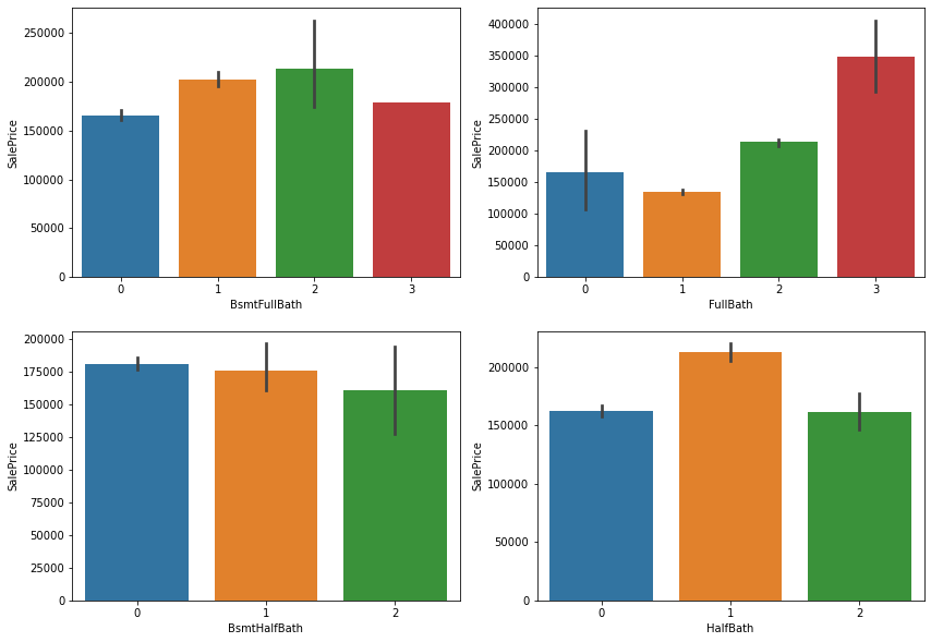
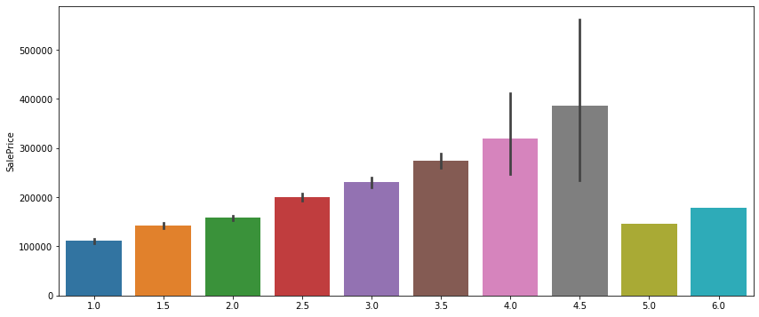
- 욕실의 개수가 증가할 수록 집값이 비싸진다
- 위에 있는 검정 선은 편차
- 맨 마지막 두개는 편차가 없는데 이는 욕실이 5,6개인 집은 각각 하나씩 있다는 의미로 이상치로 판단하고 지워도 됨
- 건축연도+리모델링 연도
figure, (ax1, ax2, ax3) = plt.subplots(nrows=1, ncols=3)
figure.set_size_inches(18,8)
sns.regplot(data['YearBuilt'], data['SalePrice'], ax=ax1)
sns.regplot(data['YearRemodAdd'], data['SalePrice'], ax=ax2)
sns.regplot((data['YearBuilt']+data['YearRemodAdd'])/2, data['SalePrice'], ax=ax3)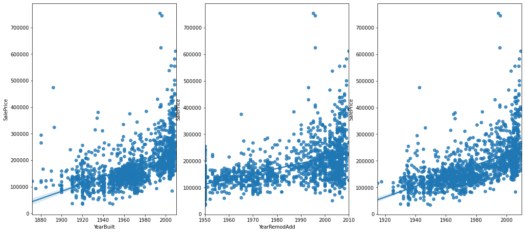
- 건축연도가 오래되었어도 최근에 리모델링을 하면 이 값이 높게 나옴
- 건축 이후 리모델링을 하지 않았다면 값 낮게 나옴
- 이 값이 높은 집들은 신축+리모델링에 가까움
all_data['YrBltAndRemod']=all_data['YearBuilt']+all_data['YearRemodAdd']all_data['MSSubClass']=all_data['MSSubClass'].astype(str)
all_data['MoSold']=all_data['MoSold'].astype(str)
all_data['YrSold']=all_data['YrSold'].astype(str)- 지하실 점수
Basement = ['BsmtCond', 'BsmtExposure', 'BsmtFinSF1', 'BsmtFinSF2', 'BsmtFinType1', 'BsmtFinType2', 'BsmtQual', 'BsmtUnfSF', 'TotalBsmtSF']
Bsmt=all_data[Basement]
#좋은 값에는 높은 숫자, 안좋은 값에는 낮은숫자, 지하실 없으면 0
Bsmt=Bsmt.replace(to_replace='Po', value=1)
Bsmt=Bsmt.replace(to_replace='Fa', value=2)
Bsmt=Bsmt.replace(to_replace='TA', value=3)
Bsmt=Bsmt.replace(to_replace='Gd', value=4)
Bsmt=Bsmt.replace(to_replace='Ex', value=5)
Bsmt=Bsmt.replace(to_replace='None', value=0)
Bsmt=Bsmt.replace(to_replace='No', value=1)
Bsmt=Bsmt.replace(to_replace='Mn', value=2)
Bsmt=Bsmt.replace(to_replace='Av', value=3)
Bsmt=Bsmt.replace(to_replace='Gd', value=4)
Bsmt=Bsmt.replace(to_replace='Unf', value=1)
Bsmt=Bsmt.replace(to_replace='LwQ', value=2)
Bsmt=Bsmt.replace(to_replace='Rec', value=3)
Bsmt=Bsmt.replace(to_replace='BLQ', value=4)
Bsmt=Bsmt.replace(to_replace='ALQ', value=5)
Bsmt=Bsmt.replace(to_replace='GLQ', value=6)Bsmt['BsmtScore']= Bsmt['BsmtQual'] * Bsmt['BsmtCond'] * Bsmt['TotalBsmtSF']
all_data['BsmtScore']=Bsmt['BsmtScore']
Bsmt['BsmtFin'] = (Bsmt['BsmtFinSF1'] * Bsmt['BsmtFinType1']) + (Bsmt['BsmtFinSF2'] * Bsmt['BsmtFinType2'])#지하실 완성도 점수
all_data['BsmtFinScore']=Bsmt['BsmtFin'] #지하실 완성도 점수
all_data['BsmtDNF']=(all_data['BsmtFinScore']==0) #지하실 미완성 여부- 토지 점수
lot=['LotFrontage', 'LotArea','LotConfig','LotShape']
Lot=all_data[lot]

Lot['LotScore'] = np.log((Lot['LotFrontage'] * Lot['LotArea'])+1)

all_data['LotScore']=Lot['LotScore']- 차고 점수
garage=['GarageArea','GarageCars','GarageCond','GarageFinish','GarageQual','GarageType','GarageYrBlt']
Garage=all_data[garage]
all_data['NoGarage']=(all_data['GarageArea']==0)Garage=Garage.replace(to_replace='Po', value=1)
Garage=Garage.replace(to_replace='Fa', value=2)
Garage=Garage.replace(to_replace='TA', value=3)
Garage=Garage.replace(to_replace='Gd', value=4)
Garage=Garage.replace(to_replace='Ex', value=5)
Garage=Garage.replace(to_replace='None', value=0)
Garage=Garage.replace(to_replace='Unf', value=1)
Garage=Garage.replace(to_replace='RFn', value=2)
Garage=Garage.replace(to_replace='Fin', value=3)
Garage=Garage.replace(to_replace='CarPort', value=1)
Garage=Garage.replace(to_replace='Basment', value=4)
Garage=Garage.replace(to_replace='Detchd', value=2)
Garage=Garage.replace(to_replace='2Types', value=3)
Garage=Garage.replace(to_replace='Basement', value=5)
Garage=Garage.replace(to_replace='Attchd', value=6)
Garage=Garage.replace(to_replace='BuiltIn', value=7)
Garage['GarageScore']=(Garage['GarageArea']) * (Garage['GarageCars']) * (Garage['GarageFinish']) * (Garage['GarageQual']) * (Garage['GarageType'])
all_data['GarageScore']=Garage['GarageScore']지하실 점수와 같은 방법으로 구함
- 기타 변수
- 비정상적으로 하나의 값만 많은 변수들 삭제
all_data=all_data.drop(columns=['Street','Utilities','Condition2','RoofMatl','Heating'])- 비정상적으로 빈 값이 많은 변수들 삭제
all_data=all_data.drop(columns=['PoolArea','PoolQC'])
all_data=all_data.drop(columns=['MiscVal','MiscFeature'])- 결측치가 많은 경우 삭제
all_data['NoLowQual']=(all_data['LowQualFinSF']==0)
all_data['NoOpenPorch']=(all_data['OpenPorchSF']==0)
all_data['NoWoodDeck']=(all_data['WoodDeckSF']==0)
전처리
- 범주형 변수
non_numeric=all_data.select_dtypes(np.object)

def onehot(col_list):
    global all_data
    while len(col_list) !=0:
        col=col_list.pop(0)
        data_encoded=pd.get_dummies(all_data[col], prefix=col)
        all_data=pd.merge(all_data, data_encoded, on='Id')
        all_data=all_data.drop(columns=col)
    print(all_data.shape)

onehot(list(non_numeric))
(2917, 308)
- 원 핫 인코딩 사용
- 데이터를 수많은 0과 한개의 1의 값으로 데이터를 구별하는 인코딩
- 수치형 변수
- 수치형 변수는 비대칭이 너무 심해지지 않게끔, Right Skewed 가 크게 되어있는 데이터들에만 로그를 씌워 적절히 변형시켜준다.
numeric=all_data.select_dtypes(np.number)

def log_transform(col_list):
    transformed_col=[]
    while len(col_list)!=0:
        col=col_list.pop(0)
        if all_data[col].skew() > 0.5:
            all_data[col]=np.log(all_data[col]+1)
            transformed_col.append(col)
        else:
            pass
    print(f"{len(transformed_col)} features had been tranformed")
    print(all_data.shape)

log_transform(list(numeric))
머신러닝 모델로 학습
from sklearn.linear_model import ElasticNet, Lasso
from sklearn.ensemble import GradientBoostingRegressor
from sklearn.pipeline import make_pipeline
from sklearn.preprocessing import RobustScaler
from xgboost import XGBRegressor
import time
import optuna
from sklearn.model_selection import cross_val_score
from sklearn.metrics import mean_squared_errormodel_Lasso= make_pipeline(RobustScaler(), Lasso(alpha =0.000327, random_state=18))
model_ENet = make_pipeline(RobustScaler(), ElasticNet(alpha=0.00052, l1_ratio=0.70654, random_state=18))
model_GBoost = GradientBoostingRegressor(n_estimators=3000, learning_rate=0.05, max_depth=4, max_features='sqrt', min_samples_leaf=15,
min_samples_split=10, loss='huber', random_state=18)- Lasso, ElasticNet, sklearn의 GradientBoosting 3 개의 모델을 불러와서 저장
- 최종 예측 결과물은 이 3개의 모델의 예측값의 평균값 사용
model_Lasso.fit(Xtrain, Ytrain)
Lasso_predictions=model_Lasso.predict(Xtest)
train_Lasso=model_Lasso.predict(Xtrain)

model_ENet.fit(Xtrain, Ytrain)
ENet_predictions=model_ENet.predict(Xtest)
train_ENet=model_ENet.predict(Xtrain)

model_XGB.fit(Xtrain, Ytrain)
XGB_predictions=model_XGB.predict(Xtest)
train_XGB=model_XGB.predict(Xtrain)

log_train_predictions = (train_Lasso + train_ENet + train_XGB )/3
train_score=np.sqrt(mean_squared_error(Ytrain, log_train_predictions))
print(f"Scoring with train data : {train_score}")

log_predictions=(Lasso_predictions + ENet_predictions + XGB_predictions ) / 3
predictions=np.exp(log_predictions)-1
submission['SalePrice']=predictions
submission.to_csv('Result.csv')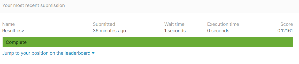
오류
XGBoost 사용시 XGBoostError
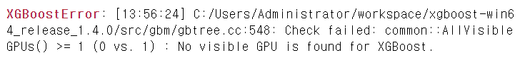
해결방법 아직 못찾아서 빼고 3개 모델들 간 평균 구함