210708 데이터 청년 캠퍼스 kaggle 실습
참고
데이터 가져오기
train=pd.read_csv("./data_in/walmart/train.csv")
features=pd.read_csv("./data_in/walmart/features.csv")
stores=pd.read_csv("./data_in/walmart/stores.csv")
test=pd.read_csv("./data_in/walmart/test.csv")train.head(2)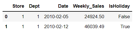
train.Date = pd.to_datetime(train.Date)
test.Date = pd.to_datetime(test.Date)features.head(2)
stores.head(2)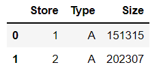
- 상점 번호, 상점 유형, 각 상점의 크기
데이터셋을 합친다
features_stores=features.merge(stores,how='inner', on=['Store'])
features_stores.Date=pd.to_datetime(features_stores.Date)
data=train.merge(features_stores,how='inner', on=['Store','Date','IsHoliday']).sort_values(by=['Store','Dept','Date']).reset_index(drop=True)

test_data = test.merge(features_stores, how='inner', on=['Store','Date','IsHoliday']).sort_values(by=['Store',
                                                                            'Dept',
'Date']).reset_index(drop=True)data.head(2)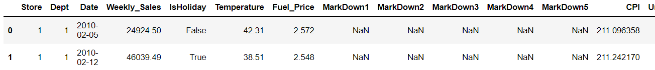
데이터 분석
휴일- 휴일 여부
data['IsHoliday'].value_counts()

plt.title('Count of Holidays')
sns.countplot(data['IsHoliday'])
plt.show()
- 휴일의 수보다 휴일이 아닌 날의 수가 더 많은 것 확인 가능
휴일 - 휴일과 휴일이 아닌 날의 판매량 비교
plt.title("Weekly sales on Holiday/Non-Holiday days")
splot=sns.barplot(x='IsHoliday', y='Weekly_Sales', data=data)
annotate_horizontal(splot)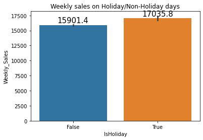
- 휴일에 판매량이 더 높은 것을 알 수 있다
plt.figure(figsize=(20,6))
plt.title("Weekly_sales box plt")
sns.boxplot(data['Weekly_Sales'])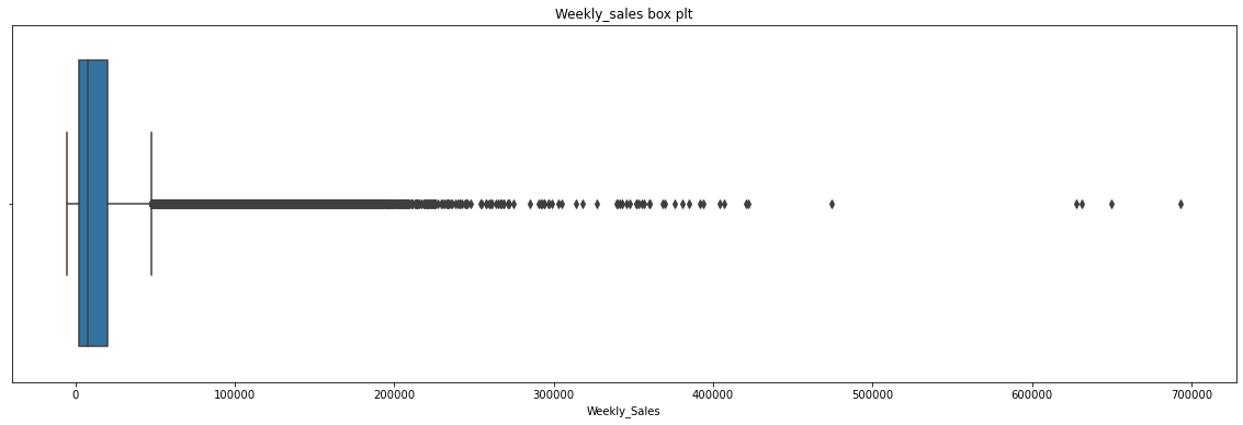
- 대부분의 판매량은 약 100000~400000이고 가장 높을 때는 600000인데 이는 휴일 일 것으로 예측 가능
data.loc[data['Weekly_Sales']>600000]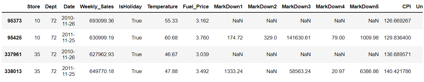
- 앞서 말한 600000이 넘는 날을 구해본 결과 4일이 있는데 이 날을 보면 ThanksGiving day로 실제로 휴일임을 알 수 있다
부서 - 각 부서 별 주간 판매량
plt.figure(figsize=(24,6))
plt.title("Weekly sales w.r.t Department")
splot=sns.barplot(x='Dept', y='Weekly_Sales', data=data)
annotate_vertical(splot)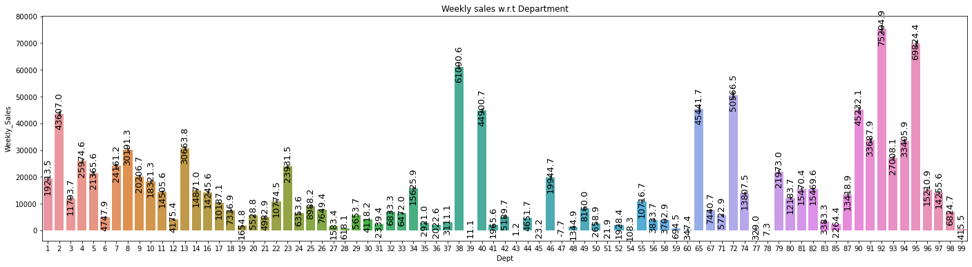
- 대부분의 부서들이 주간 판매 기록이 높은 것을 알 수 있다
plt.figure(figsize=(20,6))
plt.title("Size of each department")
splot=sns.barplot(x='Dept', y='Size', data=data)
annotate_vertical(splot)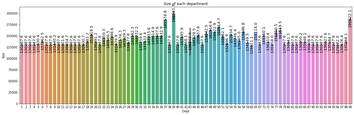
- 부서별로 판매량의 차이는 있었지만, 부서의 크기는 거의 동일하며 높은 기록을 가졌다고 부서의 크기가 무조건 큰 것은 아님을 알 수 있다
- 부서 번호 38, 92, 95를 보면 이 셋의 판매량이 가자 높지만, 이 셋의 부서의 크기가 가장 크지는 않다.
상점별 주간 판매량
plt.figure(figsize=(20,6))
plt.title("Weekly sales w.r.t Store")
splot=sns.barplot(x='Store', y='Weekly_Sales', data=data)
annotate_vertical(splot)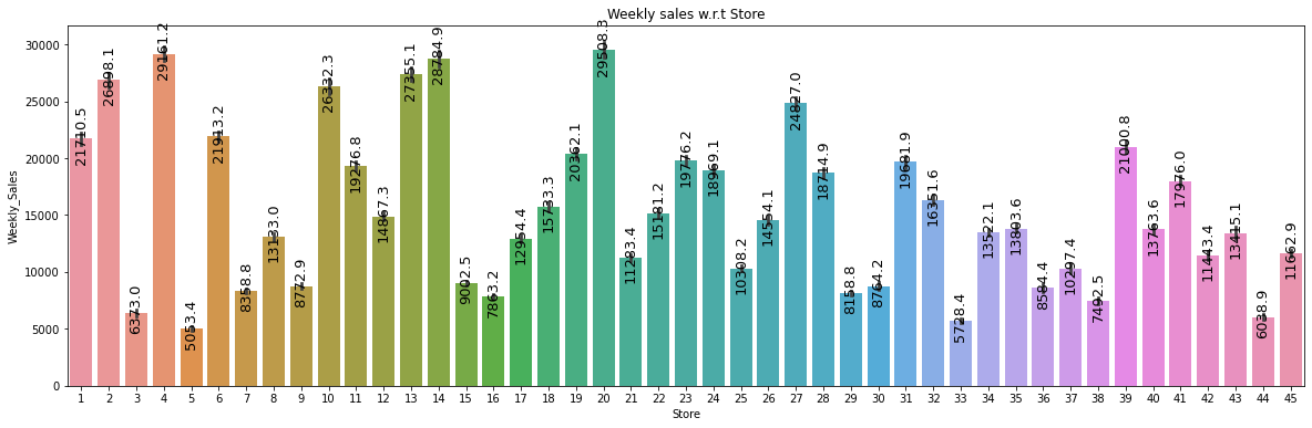
상점 크기별 판매량
plt.figure(figsize=(20,6))
plt.title("Weekly sales w.r.t Department")
plt.xticks(rotation='vertical')
splot=sns.barplot(x='Size', y='Weekly_Sales', data=data)
annotate_vertical(splot)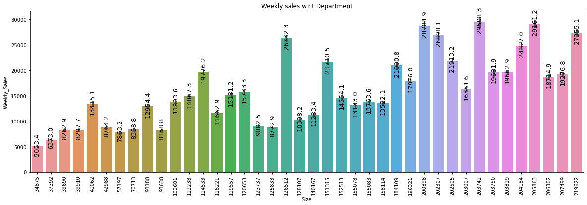
상점 유형별 비율
plt.figure(figsize=(14,8))
plt.title("Box plot between Type and Size of stores")
sns.boxplot(x='Type', y='Size',data=data)
plt.show()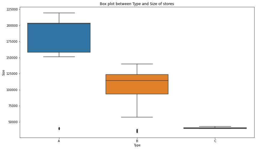
sums = data['Type'].value_counts()
plt.figure(figsize=(16,8))
#ax.axis('equal')
plt.title("Proportion of Store types")
plt.pie(sums, labels=sums.index,autopct='%1.2f%%');
plt.show()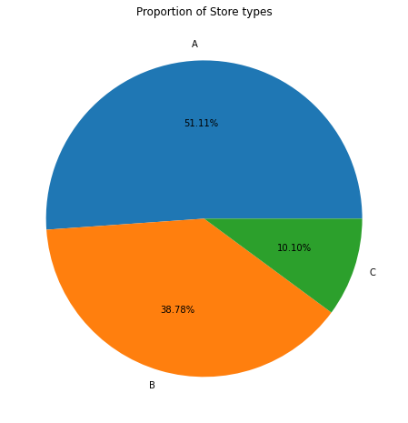
- 상점의 유형을 A, B, C로 나눠둠
- A유형이 반 이상을 차지할 정도로 매우 많은 것을 알 수 있다
상점 유형별 판매량
plt.title("Weekly_sales w.r.t Type of stores")
splot=sns.barplot(x='Type', y='Weekly_Sales', data=data)
annotate_horizontal(splot)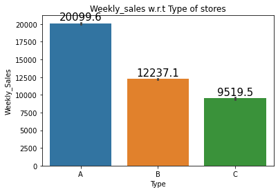
- 유형별 상점의 비율이 높을 수록 판매량이 높아지는 것을 알 수 있다.
plt.figure(figsize=(14,8))
plt.title("Box plot between weekly sales and store type")
sns.boxplot(x='Type', y='Weekly_Sales',data=data,showfliers=False)
plt.show()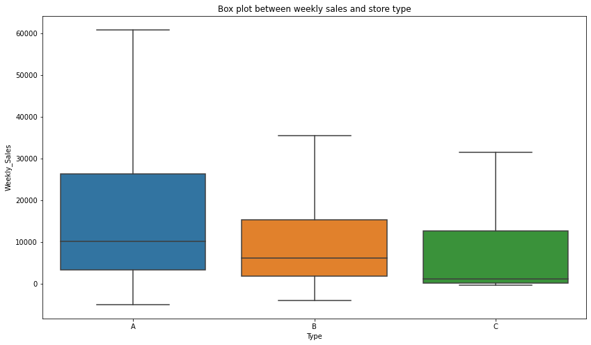
- boxplot을 보면 알 수 있듯이 A 유형의 상점이 다른 유형들보다 더 높은 판매량 기록함과 동시에 중간값도 높은 것을 알 수 있다
주간 판매량 분포
sns.FacetGrid(data, height=7).map(sns.distplot, "Weekly_Sales").add_legend();
plt.title("Distribution of Weekly_sales")
plt.show()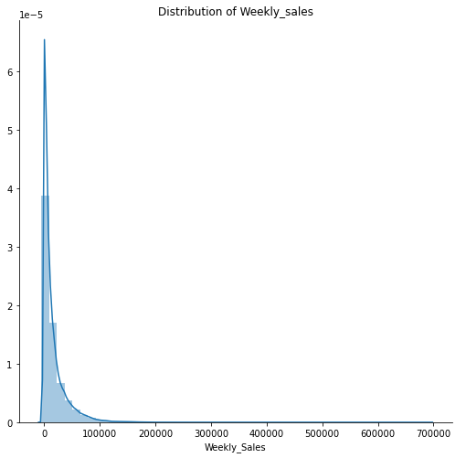
- 대부분의 판매량이 0~100000으로 기록
sns.set_style('dark')
corr = data.corr()
f,ax = plt.subplots(figsize=(20,15))
fig = sns.heatmap(corr, annot=True,linewidths=.2, cbar_kws={"shrink": .5})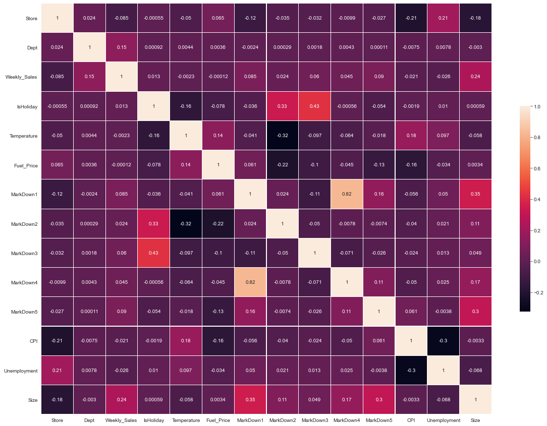
- 히트맵을 보면 온도도 판매량에 영향을 미치는 것을 알 수 있다. 너무 춥거나 더우면 판매량이 적어진다
결측값 수정
data=data.fillna(0)- 결측값을 0으로 채워준다
월간 주차별 판매량
data['Date']=pd.to_datetime(data.Date)
data['Year']=pd.DatetimeIndex(data['Date']).year
data['Month']=pd.DatetimeIndex(data['Date']).month
data['Day']=pd.DatetimeIndex(data['Date']).day
data['Day_of_year']=pd.DatetimeIndex(data['Date']).dayofyear
data['Week_of_year']=pd.DatetimeIndex(data['Date']).weekofyear

data['Month_start']=pd.DatetimeIndex(data['Date']).is_month_start
data['Month_end']=pd.DatetimeIndex(data['Date']).is_month_endtest_data['Date']=pd.to_datetime(test_data.Date)
test_data['Year']=pd.DatetimeIndex(test_data['Date']).year
test_data['Month']=pd.DatetimeIndex(test_data['Date']).month
test_data['Day']=pd.DatetimeIndex(test_data['Date']).day
test_data['Day_of_year']=pd.DatetimeIndex(test_data['Date']).dayofyear
test_data['Week_of_year']=pd.DatetimeIndex(test_data['Date']).weekofyear
test_data['Month_start']=pd.DatetimeIndex(test_data['Date']).is_month_start
test_data['Month_end']=pd.DatetimeIndex(test_data['Date']).is_month_endplt.figure(figsize=(20,6))
plt.title("Weekly sales")
splot=sns.barplot(x='week_in_month', y='Weekly_Sales', data=data)
annotate_horizontal(splot)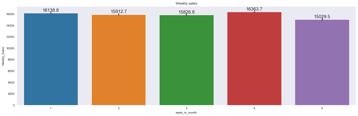
- 네번째 주의 판매량이 제일 높지만, 다른 주들과 비교했을 때 큰 차이는 없다
월간 판매량
plt.figure(figsize=(14,8))
splot=sns.barplot(data['Month'], data['Weekly_Sales'])
annotate_horizontal(splot)
plt.title("Bar plot for weeklt sales w.r.t Month")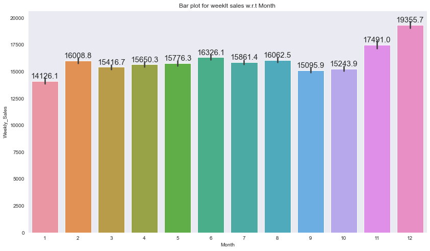
- 11월 12월이 다른 달에 비해 높게 나타남
연간 판매량
plt.title("Sales Each year")
splot=sns.barplot(data['Year'], data['Weekly_Sales'])
annotate_horizontal(splot)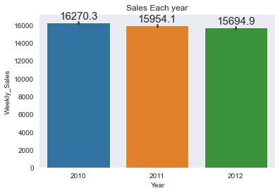
- 연간 판매량은 큰 차이가 없다
연간 주별 판매량
plt.figure(figsize=(16,7))
plt.title("Sales w.r.t each week")
splot=sns.barplot(x='Week_of_year', y='Weekly_Sales',data=data)
annotate_vertical(splot)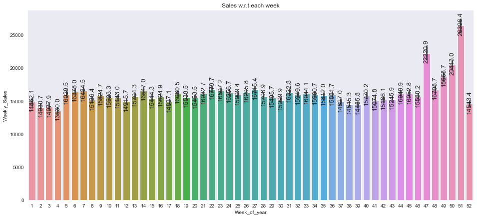
- 크리스마스와 Thanksgiving day가 있는 주에 높다
온도별 판매량
plt.figure(figsize=(16,8))
plt.scatter(data['Temperature'], data['Weekly_Sales'])
plt.title("Effect of temperatire over weekly sales")
plt.show()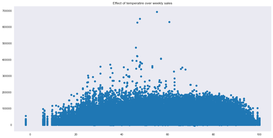
- 온도가 적절할 때에는 판매량이 높지만 너무 높거나 낮을 때에는 판매량이 낮다
모델 빌딩
data.shape, test_data.shape((421570, 28), (115064, 27))
data.head(2)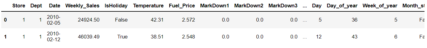
몇몇 data를 int형으로 바꿈. 이를 data와 test_date에 적용.
- 상점 유형 : A=3 / B=2/ C=1
- 휴일 유뮤 : isHoliday True = 1 / False = 0
data.Type = data.Type.apply(lambda x: 3 if x == 'A' else(2 if x == 'B' else 1))
test_data.Type = test_data.Type.apply(lambda x: 3 if x == 'A' else(2 if x == 'B' else 1))

data.IsHoliday= data.IsHoliday.apply(lambda x: 0 if x== False else 1)
test_data.IsHoliday=test_data.IsHoliday.apply(lambda x:0 if x==False else 1)
- 결측 값 확인
print(data.isnull().sum())

print("*"*50)

print(test_data.isnull().sum())
Store 0
Dept 0
Date 0
Weekly_Sales 0
IsHoliday 0
Temperature 0
Fuel_Price 0
MarkDown1 0
MarkDown2 0
MarkDown3 0
MarkDown4 0
MarkDown5 0
CPI 0
Unemployment 0
Type 0
Size 0
Year 0
Month 0
Day 0
Day_of_year 0
Week_of_year 0
Month_start 0
Month_end 0
week_in_month 0
Super_Bowl 0
Labor_day 0
Thanksgiving 0
Christmas 0
dtype: int64
Store 0
Dept 0
Date 0
IsHoliday 0
Temperature 0
Fuel_Price 0
MarkDown1 0
MarkDown2 0
MarkDown3 0
MarkDown4 0
MarkDown5 0
CPI 0
Unemployment 0
Type 0
Size 0
Year 0
Month 0
Day 0
Day_of_year 0
Week_of_year 0
Month_start 0
Month_end 0
week_in_month 0
Super_Bowl 0
Labor_day 0
Thanksgiving 0
Christmas 0
dtype: int64
data.to_csv('Train_data.csv',index=False)
test_data.to_csv('Test_data.csv', index=False)
data=pd.read_csv('Train_data.csv')
test_data=pd.read_csv('Test_data.csv')
data.columns
Index(['Store', 'Dept', 'Date', 'Weekly_Sales', 'IsHoliday', 'Temperature',
'Fuel_Price', 'MarkDown1', 'MarkDown2', 'MarkDown3', 'MarkDown4',
'MarkDown5', 'CPI', 'Unemployment', 'Type', 'Size', 'Year', 'Month',
'Day', 'Day_of_year', 'Week_of_year', 'Month_start', 'Month_end',
'week_in_month', 'Super_Bowl', 'Labor_day', 'Thanksgiving',
'Christmas'],
dtype='object')
상관관계가 없어 보이는 열을 버림. 사용하는 데이터
- store
- Dept
- Month
- Year
- Day
- Temperature
- IsHoliday
- Size
- Type
train_data_final = data.drop(columns=['CPI','Unemployment',
                          'Day_of_year','Week_of_year',
                          'Month_start','Month_end','week_in_month','Fuel_Price','MarkDown1','MarkDown2','MarkDown3',
                                      'MarkDown4','MarkDown5',
   'Super_Bowl', 'Labor_day', 'Thanksgiving',
       'Christmas'                                 ])
test_data_final = test_data.drop(columns=['CPI','Unemployment',
                          'Day_of_year','Week_of_year',
                          'Month_start','Month_end','week_in_month','Fuel_Price','MarkDown1','MarkDown2','MarkDown3',
                                          'MarkDown4','MarkDown5',
            'Super_Bowl', 'Labor_day', 'Thanksgiving',
       'Christmas'                             ])
y = train_data_final['Weekly_Sales']
X = train_data_final.drop(['Weekly_Sales'], axis=1)
train data와 test data 나누기
X_train, X_test, y_train, y_test = train_test_split(X, y, test_size=0.20, shuffle=True, random_state=42) # Train:Test = 70:20 splitting.
print(len(X_train), len(y_train), len(X_test), len(y_test))
337256 337256 84314 84314
X_train.drop(labels='Date', axis=1, inplace=True)
X_test.drop(labels='Date', axis=1, inplace=True)
from sklearn.metrics import mean_absolute_error
from sklearn.linear_model import LinearRegression
from sklearn.metrics import r2_score
from sklearn.model_selection import GridSearchCV, RandomizedSearchCV
from sklearn.svm import SVR
from sklearn.ensemble import RandomForestRegressor
from sklearn.tree import DecisionTreeRegressor
from xgboost import XGBRegressor
오류율 측정 하는 함수 성능 측정 지표 MAE를 조금 바꿔서 사용, 공휴일 무게는 5이고 나머지 날은 1로 함.
- (개인적인 추측: 공유일에 5를 둔 이유는 공유일에 판매율이 높았기 때문이 아닐까...)
def wmae(dataset, real, predicted):
    weights = dataset.IsHoliday.apply(lambda x: 5 if x else 1)
    return np.round(np.sum(weights*abs(np.array(real)-np.array(predicted)))/(np.sum(weights)), 2)
선형 회귀
regressor = LinearRegression(fit_intercept=True)
regressor.fit(X_train,y_train)

wmae(X_test, y_test, regressor.predict(X_test) )
14860.76
predictions_regressor=regressor.predict(test_data_final)
submission = pd.DataFrame({
        "Id": test_data.Store.astype(str)+'_'+test_data.Dept.astype(str)+'_'+test_data.Date.astype(str),
        "Weekly_Sales": predictions_regressor
    })

submission.to_csv('Submission_regressor.csv', index=False)
Decision Trees
#Approach of hyperparameter tuning few parameters at once is taken from below website
#<https://www.analyticsvidhya.com/blog/2016/03/complete-guide-parameter-tuning-xgboost-with-codes-python/>
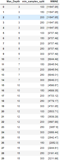
def decision_tree1(max_depth, min_samples_split):
result = []
for depth in max_depth:
for min_sample_split in min_samples_split:
wmae_test = []
#print('max_depth:', depth, ', min_samples_split:', min_sample_split)
DT = DecisionTreeRegressor(max_depth=depth, min_samples_split=min_sample_split)
DT.fit(X_train, y_train)
predicted = DT.predict(X_test)
wmae_test.append(wmae(X_test, y_test, predicted))
# print('WMAE:', wmae_test)
result.append({'Max_Depth': depth, 'min_samples_split': min_sample_split, 'WMAE': wmae_test})
return pd.DataFrame(result)
max_depth=[3,5,7,10,12,15]
min_samples_split=[100,150,200,250,300]

decision_tree1(max_depth, min_samples_split)
def decision_tree2(max_depth, min_samples_split, max_features):
    result = []
    for depth in max_depth:
        for min_sample_split in min_samples_split:
            for features in max_features:
                wmae_test = []

                #print('max_depth:', depth, ', min_samples_split:', min_sample_split)

                DT = DecisionTreeRegressor(max_depth=depth, min_samples_split=min_sample_split,
                                           max_features=features)
                DT.fit(X_train, y_train)
                predicted = DT.predict(X_test)
                wmae_test.append(wmae(X_test, y_test, predicted))
               #print('WMAE:', wmae_test)
                result.append({'Max_Depth': depth, 'min_samples_split': min_sample_split,'max_features':features, 'WMAE': wmae_test})
    return pd.DataFrame(result)
max_features=[2,3,4,5,6,7,8,9]
decision_tree2([15],[100],max_features)
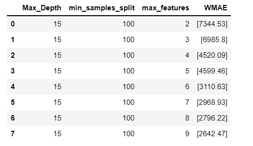
오차값 확인
final_rf=DecisionTreeRegressor(max_depth=15, min_samples_split=100,
                                           max_features=9).fit(X_train, y_train)

wmae(X_test, y_test, final_rf.predict(X_test)) #오차 결과값
2642.47
predictions_DecisionTree=final_rf.predict(test_data_final)
submission = pd.DataFrame({
        "Id": test_data.Store.astype(str)+'_'+test_data.Dept.astype(str)+'_'+test_data.Date.astype(str),
        "Weekly_Sales": predictions_DecisionTree
    })

submission.to_csv('Submission_DecisionTree.csv', index=False)
Random Forest Tree
- 우리가 만든 임의의 함수 WMAE는 Sklearn에서 정의 된 메트릭이 아니기 때문에 여기서 Gridsearch / Randomsearch를 사용할 수 없다.
- 따라서 moel에 대한 매개 변수를 취하고 각 매개 변수에 대한 wmae 점수를 표시하는 함수를 만들었다.
- 이전 블록에서 매개 변수를 가져와 추가 매개 변수와 함께 현재 블록으로 전달하는 세 가지 다른 함수를 정의했다.
def Random_forest1(n_estimators, max_depth):
    result = []
    for estimator in n_estimators:
        for depth in max_depth:

            wmae_test = []
            RF = RandomForestRegressor(n_estimators=estimator, max_depth=depth, n_jobs=8)
            RF.fit(X_train, y_train)
            predicted = RF.predict(X_test)
            wmae_test.append(wmae(X_test, y_test, predicted))
            print('n_estimators:', estimator, ', max_depth:', depth,'WMAE:', wmae_test)
            result.append({'n_estiamtors':estimator, 'Max_Depth': depth, 'WMAE': wmae_test})

    return pd.DataFrame(result)
n_estimators=[30,50,60,100,120]
max_depth=[30,35,40,45,50,60]

results=Random_forest1(n_estimators, max_depth)

#print(results)
n_estimators: 30 , max_depth: 30 WMAE: [1545.63]
n_estimators: 30 , max_depth: 35 WMAE: [1554.72]
n_estimators: 30 , max_depth: 40 WMAE: [1557.69]
n_estimators: 30 , max_depth: 45 WMAE: [1543.36]
n_estimators: 30 , max_depth: 50 WMAE: [1550.63]
n_estimators: 30 , max_depth: 60 WMAE: [1541.57]
n_estimators: 50 , max_depth: 30 WMAE: [1531.76]
n_estimators: 50 , max_depth: 35 WMAE: [1532.08]
n_estimators: 50 , max_depth: 40 WMAE: [1539.75]
n_estimators: 50 , max_depth: 45 WMAE: [1526.83]
n_estimators: 50 , max_depth: 50 WMAE: [1531.38]
n_estimators: 50 , max_depth: 60 WMAE: [1533.19]
n_estimators: 60 , max_depth: 30 WMAE: [1532.27]
n_estimators: 60 , max_depth: 35 WMAE: [1536.47]
n_estimators: 60 , max_depth: 40 WMAE: [1528.92]
n_estimators: 60 , max_depth: 45 WMAE: [1526.36]
n_estimators: 60 , max_depth: 50 WMAE: [1533.81]
n_estimators: 60 , max_depth: 60 WMAE: [1532.97]
n_estimators: 100 , max_depth: 30 WMAE: [1527.48]
n_estimators: 100 , max_depth: 35 WMAE: [1528.72]
n_estimators: 100 , max_depth: 40 WMAE: [1524.73]
n_estimators: 100 , max_depth: 45 WMAE: [1527.06]
n_estimators: 100 , max_depth: 50 WMAE: [1522.92]
n_estimators: 100 , max_depth: 60 WMAE: [1526.32]
n_estimators: 120 , max_depth: 30 WMAE: [1517.94]
n_estimators: 120 , max_depth: 35 WMAE: [1520.53]
n_estimators: 120 , max_depth: 40 WMAE: [1518.01]
n_estimators: 120 , max_depth: 45 WMAE: [1520.57]
n_estimators: 120 , max_depth: 50 WMAE: [1522.87]
n_estimators: 120 , max_depth: 60 WMAE: [1519.1]
def Random_forest2(n_estimators, max_depth,max_features):
    result = []
    for estimator in n_estimators:
        for depth in max_depth:
            for features in max_features:

                wmae_test = []
                RF = RandomForestRegressor(n_estimators=estimator, max_depth=depth,max_features=features, n_jobs=8)
                RF.fit(X_train, y_train)
                predicted = RF.predict(X_test)
                wmae_test.append(wmae(X_test, y_test, predicted))
                print('n_estimators: ',estimator,'max_depth: ',depth,'max_features:', features,'WMAE:', wmae_test)
                result.append({'n_estiamtors':estimator, 'Max_Depth': depth,'Max_Features': features, 'WMAE': wmae_test})

    return pd.DataFrame(result)
def random_forest_3(n_estimators, max_depth, max_features, min_samples_split, min_samples_leaf):
    result = []
    for features in max_features:
        for split in min_samples_split:
            for leaf in min_samples_leaf:
                wmae_test=[]
               # print('min_samples_split:', split, ', min_samples_leaf:', leaf)

                RF = RandomForestRegressor(n_estimators=n_estimators, max_depth=max_depth, max_features=features,
                                           min_samples_leaf=leaf, min_samples_split=split)
                RF.fit(X_train, y_train)
                predicted = RF.predict(X_test)
                wmae_test.append(wmae(X_test, y_test, predicted))
                print('Max_features: ', features, 'min_samples_split:', split, ', min_samples_leaf:', leaf,'WMAE:', wmae_test)
                result.append({'n_estimators':n_estimators, 'Max_Depth': max_depth,'Max_Features': max_features,
                           'min_samples_split':split,'min_samples_leaf':leaf,'WMAE': wmae_test})
    return pd.DataFrame(result)
max_features=[7,8]
min_samples_split=[2,5,7]
min_samples_leaf=[1,2,3]

result=random_forest_3(120,45,max_features,min_samples_split, min_samples_leaf)

#print(result)
Max_features: 7 min_samples_split: 2 , min_samples_leaf: 1 WMAE: [1511.46]
Max_features: 7 min_samples_split: 2 , min_samples_leaf: 2 WMAE: [1546.33]
Max_features: 7 min_samples_split: 2 , min_samples_leaf: 3 WMAE: [1593.57]
Max_features: 7 min_samples_split: 5 , min_samples_leaf: 1 WMAE: [1536.77]
Max_features: 7 min_samples_split: 5 , min_samples_leaf: 2 WMAE: [1547.28]
Max_features: 7 min_samples_split: 5 , min_samples_leaf: 3 WMAE: [1590.41]
Max_features: 7 min_samples_split: 7 , min_samples_leaf: 1 WMAE: [1572.58]
Max_features: 7 min_samples_split: 7 , min_samples_leaf: 2 WMAE: [1573.06]
Max_features: 7 min_samples_split: 7 , min_samples_leaf: 3 WMAE: [1599.53]
Max_features: 8 min_samples_split: 2 , min_samples_leaf: 1 WMAE: [1501.8]
Max_features: 8 min_samples_split: 2 , min_samples_leaf: 2 WMAE: [1537.77]
Max_features: 8 min_samples_split: 2 , min_samples_leaf: 3 WMAE: [1584.04]
Max_features: 8 min_samples_split: 5 , min_samples_leaf: 1 WMAE: [1533.78]
Max_features: 8 min_samples_split: 5 , min_samples_leaf: 2 WMAE: [1541.66]
Max_features: 8 min_samples_split: 5 , min_samples_leaf: 3 WMAE: [1578.11]
Max_features: 8 min_samples_split: 7 , min_samples_leaf: 1 WMAE: [1558.05]
Max_features: 8 min_samples_split: 7 , min_samples_leaf: 2 WMAE: [1564.51]
Max_features: 8 min_samples_split: 7 , min_samples_leaf: 3 WMAE: [1584.9]
오차값 확인
final_rf=RandomForestRegressor(

    n_estimators=120, max_depth=45, max_features=8, min_samples_split=2, min_samples_leaf=1
).fit(X_train, y_train)

wmae(X_test, y_test, final_rf.predict(X_test)) #오차 결과값
1502.56
csv로 저장
randomForest를 csv로 만들어서 캐글에 제출
import pickle

pickle.dump(final_rf, open("final_model",'wb'))
test_data_final.drop(labels='Date', axis=1, inplace=True)

predictions=final_rf.predict(test_data_final)
submission = pd.DataFrame({
        "Id": test_data.Store.astype(str)+'_'+test_data.Dept.astype(str)+'_'+test_data.Date.astype(str),
        "Weekly_Sales": predictions
    })

submission.to_csv('Submission_random_forest.csv', index=False)
제출 결과
Random Forest

선형회귀

의사 결정 트리